Budget RAID. Testing performance. Performance of Raid 0 arrays from a single disk
If you are interested in this article, then you, apparently, have encountered or expect to soon encounter one of the following problems on your computer:
- there is clearly not enough physical volume of the hard drive, as a single logical disk. Most often this problem occurs when working with large files (video, graphics, databases);These and some other problems can be solved by creating a RAID system on your computer.
- obviously not enough performance of the hard drive. Most often, this problem occurs when working with non-linear video editing systems or when a large number of users access files on a hard drive at the same time;
- obviously not enough reliability of the hard drive. Most often, this problem occurs when you need to work with data that must never be lost or that must always be available to the user. Sad experience shows that even the most reliable equipment sometimes breaks down and, as a rule, at the most inopportune moment.
What is "RAID"?
In 1987, Patterson, Gibson, and Katz of the University of California, Berkeley published A Case for Redundant Arrays of Inexpensive Disks (RAID). This article described different types of disk arrays, abbreviated as RAID - Redundant Array of Independent (or Inexpensive) Disks (redundant array of independent (or inexpensive) drives). RAID is based on the following idea: by combining several small and / or cheap drives into an array, you can get a system that surpasses the most expensive drives in terms of volume, speed and reliability. On top of that, from the point of view of a computer, such a system looks like a single drive.We know that the MTBF of an array of drives is equal to the MTBF of a single drive divided by the number of drives in the array. As a result, the MTBF of an array is too short for many applications. However, a disk array can be made tolerant of a single drive failure in several ways.
In the above article, five types (levels) of disk arrays were defined: RAID-1, RAID-2, ..., RAID-5. Each type provided fault tolerance as well as different advantages over a single drive. Along with these five types, the non-redundant RAID-0 disk array has also become popular.
What are the RAID levels and which one should I choose?
RAID-0. Typically defined as a non-redundant drive group with no parity. RAID-0 is sometimes called "Striping" ("striped" or "vest") by the method of placing information on the drives included in the array:Since RAID-0 is not redundant, the failure of one drive causes the entire array to fail. On the other hand, RAID-0 provides maximum exchange speed and efficient use of disk space. Since RAID-0 does not require complex mathematical or logical calculations, its implementation costs are minimal.
Scope: audio and video applications requiring high speed continuous data transfer, which cannot be provided by a single drive. For example, studies conducted by Mylex to determine the optimal disk system configuration for a non-linear video editing station show that, compared to a single drive, a two-drive RAID-0 array gives a 96% increase in write / read speed from three drives - by 143% (according to the Miro VIDEO EXPERT Benchmark test).
The minimum number of drives in a "RAID-0" array is 2.
RAID-1. More commonly known as "Mirroring", it is a pair of drives that contain the same information and make up one logical drive:
Recording is done on both drives in each pair. However, the drives in a pair can perform concurrent reads. Thus "mirroring" can double the read speed, but the write speed remains the same. RAID-1 has 100% redundancy and failure of one drive does not lead to failure of the entire array - the controller simply switches read/write operations to the remaining drive.
RAID-1 provides the highest performance among all types of redundant arrays (RAID-1 - RAID-5), especially in a multi-user environment, but the worst use of disk space. Since RAID-1 does not require complex mathematical or logical calculations, its implementation costs are minimal.
The minimum number of drives in a "RAID-1" array is 2.
Multiple RAID-1 arrays can be combined into RAID-0 to increase write speed and ensure data reliability. This configuration is called "two-level" RAID or RAID-10 (RAID 0+1):
The minimum number of drives in a "RAID 0+1" array is 4.
Scope: cheap arrays, in which the main thing is the reliability of data storage.
RAID-2. Distributes data in sector-sized stripes across a group of drives. Some drives are dedicated to storing ECC (Error Correction Code). Since most drives store per-sector ECC codes by default, RAID-2 offers little advantage over RAID-3 and is therefore not widely used.
RAID-3. As in the case of RAID-2, the data is distributed over stripes of one sector in size, and one of the drives in the array is allocated for storing parity information:
RAID-3 relies on the ECC codes stored in each sector for error detection. In the event of a failure of one of the drives, restoring the information stored on it is possible by calculating exclusive OR (XOR) based on the information on the remaining drives. Each entry is usually distributed across all drives, and so this type of array is good for disk-intensive applications. Since each I/O operation accesses all the drives in the array, RAID-3 cannot perform multiple operations at the same time. Therefore, RAID-3 is good for a single-user, single-tasking environment with long writes. To work with short recordings, synchronization of the rotation of disk drives is required, since otherwise a decrease in the exchange rate is inevitable. It is rarely used, because. outperforms RAID-5 in terms of disk space usage. Implementation is costly.
The minimum number of drives in a "RAID-3" array is 3.
RAID-4. RAID-4 is identical to RAID-3 except that the stripe size is much larger than one sector. In this case, reading is from a single drive (not counting the drive that stores parity information), so multiple reads can be performed at the same time. However, since each write operation must update the contents of the parity drive, multiple write operations cannot be performed at the same time. This type of array has no noticeable advantages over a RAID-5 array.
RAID-5. This type of array is sometimes called a "rotating parity array". This type of array successfully overcomes the disadvantage inherent in RAID-4 - the inability to simultaneously perform multiple write operations. This array, like RAID-4, uses stripes big size, but, unlike RAID-4, parity information is stored not on one drive, but on all drives in turn:
Write operations access one drive with data and the other drive with parity information. Since the parity information for different stripes is stored on different drives, it is only possible to perform multiple simultaneous writes in those rare cases when either data or parity stripes are on the same drive. The more drives in the array, the less often the location of the information and parity stripes coincide.
Scope: reliable arrays of large volume. Implementation is costly.
The minimum number of drives in a "RAID-5" array is 3.
RAID-1 or RAID-5?
Compared to RAID-1, RAID-5 uses disk space more economically, since it does not store a “copy” of information for redundancy, but a control number. As a result, any number of drives can be combined in RAID-5, of which only one will contain redundant information.
But a higher efficiency of disk space use is achieved at the expense of a lower information exchange rate. While writing information to RAID-5, you need to update the parity information each time. To do this, you need to determine which parity bits have changed. First, the old information to be updated is read. This information is then multiplied by XOR with new information. The result of this operation is a bit mask, in which each bit =1 means that the parity information in the corresponding position should be replaced with a value. Then, the updated parity information is written to the appropriate location. Therefore, for every program request to write information, RAID-5 performs two reads, two writes, and two XORs.
The more efficient use of disk space (a parity block is stored instead of a copy of the data) comes at a cost: it takes extra time to generate and write parity information. This means that the write speed on RAID-5 is lower than on RAID-1 in a ratio of 3:5 or even 1:3 (i.e., the write speed on RAID-5 is 3/5 to 1/3 of the write speed RAID-1). Because of this, RAID-5 is pointless to create in software. They also cannot be recommended in cases where it is the write speed that is critical.
Which way to implement RAID - software or hardware?
Reading the descriptions of the different levels of RAID, you'll notice that nowhere are there any specific hardware requirements that are required to implement RAID. From which we can conclude that all that is needed to implement RAID is to connect the required number of drives to the controller available in the computer and install special software on the computer. This is true, but not quite!Indeed, there is the possibility of a software implementation of RAID. An example would be OS Microsoft Windows NT 4.0 Server, which can implement software RAID-0, -1, and even RAID-5 (Microsoft Windows NT 4.0 Workstation provides only RAID-0 and RAID-1). However, this solution should be considered as extremely simplified, not allowing to fully realize the capabilities of a RAID array. Suffice it to say that with a software implementation of RAID, the entire burden of placing information on disk drives, calculating control codes, etc. falls on CPU, which naturally does not increase the performance and reliability of the system. For the same reasons, there are practically no service functions here, and all operations to replace a faulty drive, add a new drive, change the RAID level, etc. are performed with a complete loss of data and with a complete ban on performing any other operations. The only advantage of a software implementation of RAID is the minimal cost.
- a specialized controller frees the CPU from basic operations with RAID, and the effectiveness of the controller is all the more noticeable, the higher the level of complexity of the RAID;The disadvantage of hardware RAID is the relatively high cost of RAID controllers. However, on the one hand, you have to pay for everything (reliability, speed, service). On the other hand, recently, with the development of microprocessor technology, the cost of RAID controllers (especially lower models) began to fall sharply and became comparable to the cost of ordinary disk controllers, which makes it possible to install RAID systems not only in expensive mainframes, but also in servers. entry level and even workstations.
- controllers, as a rule, are equipped with drivers that allow you to create a RAID for almost any popular operating system;
- the built-in BIOS of the controller and the control programs attached to it allow the system administrator to easily connect, disconnect or replace drives included in the RAID, create several RAID arrays, even of different levels, monitor the state of the disk array, etc. With "advanced" controllers, these operations can be performed "on the fly", i.e. without turning off system unit. Many operations can be performed in " background”, i.e. without interrupting the current work and even remotely, i.e. from any (of course, if you have access) workplace;
- controllers can be equipped with a buffer memory ("cache"), which stores the last few blocks of data, which, with frequent access to the same files, can significantly increase the speed of the disk system.
How to choose a RAID controller model?
There are several types of RAID controllers depending on their functionality, design and cost:1. Drive controllers with RAID functionality.
In fact, this is an ordinary disk controller, which, thanks to a special BIOS firmware, allows you to combine drives into a RAID array, usually level 0, 1 or 0 + 1.
Ultra (Ultra Wide) SCSI controller from Mylex KT930RF (KT950RF).
Externally, this controller is no different from an ordinary SCSI controller. All "specialization" is in the BIOS, which is, as it were, divided into two parts - "SCSI Configuration" / "RAID Configuration". Despite the low cost (less than $200), this controller has a good set of functions:
- Combining up to 8 drives in RAID 0, 1 or 0+1;
- support hot spare to replace "on the fly" a failed drive;
- the possibility of automatic (without operator intervention) replacement of a faulty drive;
- automatic control of integrity and identity (for RAID-1) of data;
- the presence of a password to access the BIOS;
- RAIDPlus program providing information about the status of drives in RAID;
- drivers for DOS, Windows 95, NT 3.5x, 4.0
Now let's see what types there are and how they differ.
UC Berkeley introduced the following levels of the RAID specification, which have been adopted as the de facto standard:
- RAID 0- high-performance disk array with striping, without fault tolerance;
- - mirror disk array;
- RAID 2 reserved for arrays that use Hamming code;
- RAID 3 and 4- disk arrays with striping and a dedicated parity disk;
- - disk array with striping and "unallocated parity disk";
- - striped disk array using two checksums calculated in two independent ways;
- - RAID 0 array built from RAID 1 arrays;
- - RAID 0 array built from RAID 5 arrays;
- - a RAID 0 array built from RAID 6 arrays.
A hardware RAID controller can support several different RAID arrays at the same time, the total number of hard drives of which does not exceed the number of slots for them. At the same time, the controller built into the motherboard, in BIOS settings has only two states (enabled or disabled), so a new hard drive connected to an unused controller connector when activated mode RAID may be ignored by the system until it is associated as another JBOD (spanned) RAID array consisting of a single disk.
RAID 0 (striping - "alternating")
The mode that maximizes performance. The data is evenly distributed across the disks of the array, the disks are combined into one, which can be divided into several. Distributed read and write operations allow you to significantly increase the speed of work, since several disks simultaneously read / write their portion of data. The entire volume of disks is available to the user, but this reduces the reliability of data storage, since if one of the disks fails, the array is usually destroyed and it is almost impossible to restore data. Scope - applications that require high speeds of disk exchange, such as video capture, video editing. Recommended for use with high reliability drives.

(mirroring - "mirroring")
an array of two disks that are full copies of each other. Not to be confused with RAID 1+0, RAID 0+1, and RAID 10 arrays, which use more than two drives and more sophisticated mirroring mechanisms.
Provides an acceptable write speed and a gain in read speed when parallelizing queries.
It has high reliability - it works as long as at least one disk in the array is functioning. The probability of failure of two disks at once is equal to the product of the probabilities of failure of each disk, i.e. significantly lower than the probability of failure of a single drive. In practice, if one of the disks fails, urgent measures should be taken - redundancy should be restored again. To do this, with any RAID level (except zero), it is recommended to use hot spare disks.

Similar to RAID10, a variant of data distribution across disks, allowing the use of an odd number of disks (the minimum number is 3)
RAID 2, 3, 4
various options for distributed storage with disks allocated for parity codes and various block sizes. Currently, they are practically not used due to low performance and the need to allocate a lot of disk space for storing ECC and/or parity codes.


The main disadvantage of RAID levels 2 to 4 is the inability to perform parallel write operations, since a separate parity disk is used to store parity information. RAID 5 does not have this drawback. Data blocks and checksums are cyclically written to all disks in the array, there is no asymmetry in disk configuration. Checksums are the result of an XOR operation (exclusive or). Xor has a feature that makes it possible to replace any operand with the result, and, using the algorithm xor, get the missing operand as a result. For example: a xor b = c(where a, b, c- three disks of the raid array), if a refuses, we can get him by putting him in his place c and having spent xor between c And b: xor b = a. This applies regardless of the number of operands: a xor b xor c xor d = e. If it fails c then e takes his place and xor as a result we get c: a xor b xor e xor d = c. This method essentially provides version 5 fault tolerance. It only takes 1 disk to store the xor result, the size of which is equal to the size of any other disk in the raid.
Advantages
RAID5 has become widespread, primarily due to its cost-effectiveness. The size of a RAID5 disk array is calculated using the formula (n-1)*hddsize, where n is the number of disks in the array and hddsize is the size of the smallest disk. For example, for an array of four 80 GB disks, the total volume will be (4 - 1) * 80 = 240 GB. Additional resources are spent on writing information to a RAID 5 volume and performance drops, since additional calculations and write operations are required, but when reading (compared to a separate hard drive), there is a gain, because data streams from several array disks can be processed in parallel.
disadvantages
RAID 5 performance is noticeably lower, especially on Random Write operations (writes in random order), in which performance drops by 10-25% from RAID 0 (or RAID 10) performance, since it requires more disk operations (each operation writes, with the exception of the so-called full-stripe writes, the server is replaced on the RAID controller by four - two reads and two writes). The disadvantages of RAID 5 appear when one of the disks fails - the entire volume goes into critical mode (degrade), all write and read operations are accompanied by additional manipulations, performance drops sharply. In this case, the reliability level is reduced to the reliability of RAID-0 with the appropriate number of disks (that is, n times lower than the reliability of a single disk). If a failure occurs before the array is completely restored, or an unrecoverable read error occurs on at least one more disk, then the array is destroyed, and the data on it cannot be restored by conventional methods. It should also be taken into account that the process of RAID Reconstruction (recovery of RAID data due to redundancy) after a disk failure causes an intensive read load from disks for many hours continuously, which can cause any of the remaining disks to fail in this least protected period of RAID operation, as well as to detect previously undetected read failures in cold data arrays (data that is not accessed during normal operation of the array, archived and inactive data), which increases the risk of failure during data recovery.
The minimum number of used disks is three.


RAID 6 - similar to RAID 5, but has a higher degree of reliability - the capacity of 2 disks is allocated for checksums, 2 sums are calculated using different algorithms. Requires a more powerful RAID controller. Provides operability after simultaneous failure of two disks - protection against multiple failure. A minimum of 4 disks is required to organize an array. Typically, using RAID-6 causes about a 10-15% drop in disk group performance compared to RAID 5, which is caused by a large amount of processing for the controller (the need to calculate a second checksum, and read and overwrite more disk blocks when each block is written).

RAID 0+1
RAID 0+1 can basically mean two options:
- two RAID 0s are merged into RAID 1;
- three or more disks are combined into an array, and each data block is written to two disks of this array; thus, with this approach, as in "pure" RAID 1, the useful volume of the array is half of the total volume of all disks (if these are disks of the same capacity).
RAID 10 (1+0)
RAID 10 is a mirrored array in which data is written sequentially to several disks, as in RAID 0. This architecture is a RAID 0 type array, the segments of which are RAID 1 arrays instead of individual disks. Accordingly, an array of this level must contain at least 4 disks ( and always an even number). RAID 10 combines high fault tolerance and performance.
The claim that RAID 10 is the most reliable option for data storage is justified by the fact that the array will be taken out of service after the failure of all drives in the same array. With one drive failing, the chance of failure of the second one in the same array is 1/3*100=33%. RAID 0+1 will fail if two drives fail in different arrays. The chance of failure of a drive in a neighboring array is 2/3*100=66%, however, since a drive in an array with a drive that has already failed is no longer used, the chance that the next drive will disable the entire array is 2/2 *100=100%

an array similar to RAID5, however, in addition to distributed storage of parity codes, the distribution of spare areas is used - in fact, it is used HDD, which can be added to a RAID5 array as a spare (such arrays are called 5+ or 5+spare). In a RAID 5 array, the spare drive is idle until one of the primary drives fails. hard drives, while in a RAID 5EE array, this drive is shared with the rest of the HDD all the time, which has a positive effect on the performance of the array. For example, a RAID5EE array of 5 HDDs can perform 25% more I/O operations per second than a RAID5 array of 4 primary and one spare HDD. The minimum number of disks for such an array is 4.

combining two (or more, but this is extremely rarely used) RAID5 arrays into a stripe, i.e. a combination of RAID5 and RAID0, partially correcting the main disadvantage of RAID5 - low speed writing data through the parallel use of several such arrays. The total capacity of the array is reduced by the capacity of two drives, but unlike RAID6, it can only tolerate a single drive failure without data loss, and the minimum number of drives required to create a RAID50 array is 6. Along with RAID10, this is the most recommended RAID level to use. in applications where high performance combined with acceptable reliability is required.

merging two RAID6 arrays into a stripe. The write speed is approximately double that of the write speed in RAID6. The minimum number of disks to create such an array is 8. Information is not lost if two disks from each RAID 6 array fail.

RAID 00
RAID 00 is very rare, I met it on LSI controllers. A RAID 00 disk group is a spanned disk group that creates a striped set from a series of
disk arrays RAID 0. RAID 00 does not provide data redundancy, but along with RAID 0, offers the best performance of any RAID level. RAID 00 breaks the data into smaller segments and then stripes the data segments on each disk in a storage group. The size of each data segment is determined by the stripe size. RAID 00 offers high bandwidth. RAID 00 is not fault tolerant. If a disk in a RAID 0 disk group fails, the entire
virtual disk (all disks associated with virtual disk) will fail. By splitting a large file into smaller segments, the RAID controller can use both SAS
controller to read or write a file faster. RAID 00 does not assume parity calculations complicate write operations. This makes RAID 00 ideal for
applications that require high bandwidth but do not require fault tolerance. Can consist of 2 to 256 disks.

Which is faster RAID 0 or RAID 00?

I conducted my testing described in the article about optimizing the speed of solid state drives on LSI controllers and got these numbers on arrays of 6 SSDs
Comparing the performance of solutions of the same price level
A curious fact: the so-called Experience Index in Windows 7, which evaluates the performance of the main PC subsystems, for a typical solid-state drive (SSD), and far from the slowest (around 200 MB / s for reading and writing, random access - 0.1 ms) , shows a value of 7.0, while the indexes of all other subsystems (processor, memory, graphics, game graphics) in the same desktop systems based on older CPUs (with an average of 4 GB DDR3-1333 memory for today and an average the same gaming graphics card like the AMD Radeon HD 5770) are evaluated by values significantly higher than 7.0 (namely, 7.4-7.8; this criterion in Windows 7 has a logarithmic scale, so the difference in tenths translates into tens of percent of absolute values). That is, a fast "household" SSD on the SATA bus, according to Windows 7, is the bottleneck even in not the most top-end desktop PCs of today. What should be the (outrageous?) performance of the system disk so that the "great and mighty" "Seven" consider it worthy of the rest of the components of such a PC? .. :)
This question, apparently, is rhetorical, since few people are now guided by the "experience index" of Windows 7 when selecting the configuration of their desktop. And SSDs are already firmly rooted in the minds of users as a non-alternative option, if you want to squeeze the maximum out of the disk subsystem and get a comfortable, “no brakes” work. But is it really so? Is Windows 7 alone in its assessment of the real usefulness of SSDs? And is there an alternative to SSD in powerful desktops? Especially if you don’t really want to see the hopeless emptiness in your wallet ... We dare to offer one of options replacements.
What are the main disadvantages of modern SSDs? If we do not take into account the "long-playing" disputes about their reliability, durability and degradation over time, then there are, by and large, two such shortcomings: a small capacity and a rather high price. Indeed, a mediocre 128 GB MLC SSD now costs around 8,000 rubles. (price at the time of writing; of course, it depends heavily on the model, but the order of prices is so far). This, of course, is not 600 rubles per 1 GB, as for DDR3 memory, but an order of magnitude less, but still far from so small as for traditional magnetic hard drives. Indeed, a very productive "seven-thousander" of 1000 GB with a maximum read / write speed of about 150 MB / s (which, by the way, is not much less than an SSD for 8 thousand rubles!) Now you can buy less than 2000 rubles. (for example, Hitachi 7K1000.C or something Korean). The unit cost of a gigabyte of space in this case will be only 2 (two) rubles! Do you feel the difference with the SSD with its 60 rubles per gigabyte? ;) And is the "chasm" between them really that big in typical desktop applications with a large number of consecutive accesses? For example, when working with video, audio, graphics, etc. After all, the typical sequential read speed of an MLC SSD (160-240 MB / s) does not much exceed that of the first 120 gigabytes of space in the same "seven-thousander terabyte" (150 MB / s). from). And in terms of sequential write speed, they generally have approximate parity (the same 150 MB / s versus 70-190 for SSDs). Yes, in terms of random access time, they are completely incomparable, but after all, we are not building a server for ourselves on the desktop.
Moreover, for a desktop, the same 128 GB at the present time is an extremely frivolous volume (in 80 GB it is generally ridiculous). It will barely fit one or two system partitions with the OS and main applications. And where to store numerous multimedia files? Where to put toys, each of which will now pull on 5-20 GB unpacked? In short, without a normal capacious "screw" is still nowhere. The only question is whether it will be system or additional in the computer.
What if you approach from the other side? Since without a hard drive (remember the good old abbreviation - hard disk drives, or simply "hard drives") with a PC anywhere, then why not combine them into a RAID array? Moreover, many of us got a simple RAID controller, in fact, "for free" - in the south bridge of motherboards based on AMD, Intel or Nvidia chipsets. For example, the same 8,000 rubles can be spent not on an SSD, but on 4 “terabytes”. Let's combine them into an array (s) - then we won't have to buy a capacious HDD for data storage, that is, we'll even save. Or as a second option - together with the purchase of one SSD and one 2-3 TB disk, you can purchase 4 disks of 1.5-2 TB each ...
What's more, say a four-disk RAID 0 will have not only quadruple the capacity, but also four times the read/write linear speed. And this is already 400-600 MB / s, which is a single SSD the same price didn't even dream! Thus, such an array will work much faster than an SSD, according to at least, with streaming data (reading/writing/editing video, copying large files, etc.). It is possible that in other typical problems personal computer such an array will behave no worse than an SSD - after all, the percentage of sequential operations in such tasks is very high, and random accesses, as a rule, are made on a fairly compact section of such a capacious drive (paging file, temporary photo editor file, etc.), that is, moving heads inside this section will be much faster than the average for the disk - in a couple of milliseconds), which, of course, will have a positive effect on its performance. If a multi-disk RAID array is also cached in the OS, then you can expect impressive speed from it even in operations with small data blocks.
To test our assumptions, we tested four-disk RAID 0 and RAID 5 arrays of Hitachi Deskstar E7K1000 terabyte drives with 7200 rpm and 32 MB buffer. Yes, they are somewhat slower in terms of the speed of the plates than the newer ones and those currently sold at 1800-1900 rubles per piece. Hitachi 7K1000.C drives of the same capacity. However, their firmware is better optimized for disks in arrays, therefore, having a little short of the coveted 600 MB / s for the maximum read speed of a 4-disk RAID 0, we will get better performance in tasks with a considerable number of random accesses. And the patterns we found can be extended to arrays of faster (and more capacious) disk models from different manufacturers.
Using motherboards based on Intel chipsets with ICH8R/ICH9R/ICH10R (and later) southbridges, we think it is optimal to organize four terabyte disks as follows. Thanks to Intel Matrix RAID technology, from the first half of the volume of each of the disks we make a 2 TB RAID 0 array (so that it can be understood by operating systems below Vista without special tricks), which will provide us with the highest performance of system partitions, quick launch applications and games, as well as high-speed operational work with multimedia and other content. And for more reliable storage of data that is important to us, we will combine the second half of the volume of these disks into a RAID 5 array (by the way, the performance is also far from the worst, as we will see below). Thus, for only 8 thousand rubles. we will get both a super-fast 2 TB system disk and a reliable and capacious 1.5 TB “archive” volume. It is in this configuration of the two arrays that we created with default values that we will conduct our further testing. However, especially suspicious RAID5 haters on Intel controllers can instead build a RAID10 one and a half times smaller - its performance for reading data will be lower than that of RAID5, when writing (with caching) they are approximately equivalent, but the reliability and data retrievability when the array collapses will be better (in half of the cases, RAID10 can be revived if even two disks fail).
The Intel Matrix Storage Manager utility allows you to enable and disable write caching on such disk arrays using the operating system (that is, using RAM PC), see the third line from the top in the right Information field in the screenshot:

Caching can drastically speed up the operation of arrays with small files and data blocks, as well as the speed of writing to a RAID 5 array (which is sometimes very critical). Therefore, for clarity, we conducted tests with caching enabled and disabled. For reference, we will also touch on CPU load issues with caching enabled below.
The tests were carried out by us on a test system representing a typical, not the most powerful desktop in modern times:
- processor Intel Core 2 Duo E8400 (3 GHz);
- 2 GB DDR2-800 system memory;
- ASUS P5Q-E board based on Intel P45 Express chipset with ICH10R;
- video accelerator AMD Radeon HD 5770.
The Seagate ST950042AS system drive contained Windows 7 x64 Ultimate and Windows XP SP3 Pro (tested arrays and drives were tested in a "clean" state). We used ATTO Disk Benchmark 2.41, Futuremark PCMark05, Futuremark PCMark Vantage x86, Intel NAS Performance Toolkit 1.7, etc. as benchmarks, based on the results of which we will judge the rivalry of SSDs with traditional RAID. The tests were carried out five times and the results were averaged. For orientation, at the bottom of the diagrams with test results, data is given for a fast single drive Seagate Barracuda XT ST32000641AS with a capacity of 2 TB, that is, the same as the “system” RAID 0 of the four Hitachi Deskstar E7K1000 HDE721010SLA330 tested by us.
The honor of an inexpensive, but very productive SSD with a capacity of 128 GB and a price (at the time of this writing) in the region of 8000 rubles. protected the PNY Optima SSD 128GB MLC model. Let's take a closer look at it first.
SSD PNY Optima 128GB Gen2
Model number P-SSD2S128GM-CT01 (firmware 0309) is a typical 2.5" SATA SSD in a stylish 9.5mm thick black metal case. Its manufacturer is a company better known for its flash drives and memory modules.

PNYOptimaSSD 128GBMLC
The drive is based on Intel 29F64G08CAMDB flash memory with MLC cells and a JMicron JMF612 controller, which allows this SSD to work not only via Serial ATA, but also via USB 2.0 (the latter's mini-connector is located next to the SATA port in the rear end of the disk case) .

That is, this solid state drive can also be used as a shock-resistant portable storage. True, the USB cable is not included in the package. But the price of the product can not be called overpriced.

Drive boardPNYOptimaSSD 128GBMLC
The manufacturer promises for this model a read speed of 235 MB / s and a write speed of 150 MB / s (in practice, it turned out to be even slightly higher). The disk cache is 64MB, TRIM support is built in, shock resistance is claimed at 1500g, and the operating temperature range is from -10 to +70°C. The manufacturer gives a 3-year warranty for this model with an MTBF of 1.5 million hours.
By the way, one should not be mistaken and consider the popular MLC SSDs based on the JMicron JMB612 controller as "lower grade" solutions. As shown, drives on this controller look on average no worse than SSDs of similar capacity and prices on controllers from Indilinx (IDX110), Intel, SandForce (SF1222) and Samsung, even outperforming them in a number of disk benchmarks.
Test results
The maximum sequential read and write speed of payload data for the PNY Optima 128GB SSD according to the results of the ATTO Disk Benchmark 2.41 test (writing and reading a 256 MB file in blocks from 64 KB to 8 MB) was 238 and 155 MB / s, respectively, which is slightly higher than those declared by the manufacturer values (see diagram).
Curiously, the HD Tach RW 3.0 low-level test, which uses access to the drive bypassing the file system, showed values of 217 and 165 MB/s for these two parameters, respectively (see graph). As for the pair of four-disk RAID arrays we tested, RAID 0 showed a maximum read / write speed of large files under 450 MB / s (this is also confirmed by the HD Tach RW 3.0 graph), which is two to three times faster than this SSD! True, enable write caching (WC=yes on diagrams) Windows tools somewhat reduces the speed of sequential writing, as well as reading, but not so critical that it can be considered unacceptable.
As for RAID 5, organized on the second half of our test hard drives, then maximum speed sequential reading of this array exceeds 270 MB / s (which is noticeably higher than that of any modern magnetic hard drive!), And the sequential write speed is fundamentally dependent on caching in Windows: without it, it barely reaches completely unacceptable 40-50 MB / s, then how it increases more than three times (see also the HD Tach RW 3.0 graph), although it still does not reach that when reading RAID 5, as it was with RAID 0. But in any case, here our RAID 5 works noticeably faster than a single one " seven thousandth" Seagate Barracuda XT.
Another significant benefit of Windows caching of disk arrays is a dramatic acceleration of work with small (less than 64 KB) files and data blocks. This is clearly seen from the results of the ATTO Disk Benchmark 2.41 test (the verticals on the left indicate the size of the data block in KB; the columns on the right are the speed values in KB / s).

RAID 0 without caching

RAID 0 with caching

RAID 5 without caching

RAID 5 with caching
As you can see, this speeds up work not only when writing, but also when reading. In general, the use of array caching in the OS is actually a sine qua non if you want to get good performance on them, not only with streaming data, but in everything else (like a system disk, for example).
The operation of caching operations with RAID through the computer's RAM (both when reading and writing) is clearly demonstrated by the following diagram, which we usually give as an illustration of the speed of the disk interface (SATA, SAS, etc.).
Buffered read speeds of 3-5 GB/s are in the same order of magnitude as system memory bandwidth in a PC like our tester. The DMI bus, through which the south bridge of Intel chipsets communicates with the system, has a much lower potential, which is, in fact, equal to the bus PCI Express x4 first generation (i.e. 1 GB/s in one direction). The second useful conclusion from this diagram is that for RAID arrays (even without caching), the data transfer rate over the bus (several SATA buses) from the host to the drives increases conditionally in proportion to the number of disks in the array. And for RAID 0, for example, it is many times higher than the data exchange rate with a single SSD on the SATA bus. The conclusion, in general, is quite obvious.
By the way, the average time of random access to arrays (small blocks) when reading does not depend on Windows caching, but when writing, it changes significantly (see diagram). Moreover, for the simplest (software) RAID 5 without caching, it is indecently large.
As for the issue of additional processor load from caching, it certainly exists, but for more or less modern desktops it cannot be called too burdensome. Let's take a look at the CPU usage graphs when running the same ATTO test:
 RAID 0
  RAID 5
CPU usage graphs without RAID caching
For both RAID 0 and RAID 5, read and write CPU usage without Windows RAID caching is a few percent. If caching is enabled, then on small blocks the CPU load increases to tens of percent, sometimes exceeding 50% (left parts of the graphs below).
 RAID 0
  RAID 5
CPU Load Graphs with RAID Caching
Interestingly, for RAID 5, the load on the processor is slightly lower than for RAID 0 - apparently, the higher read / write speed for the second case affects. In addition, as the data block size increases, the processor load decreases, approaching that with disabled caching for blocks of 64 KB and above. Of course, this is just an estimate, an illustration of the question. This aspect could be explored more scrupulously, in a "pure form". But in this case, this is not the purpose of the article for us, since the question that interests us here is what is the performance of the drives.
We evaluated the latter, in particular, by complex tests that simulate the work of various tasks under Windows - PCMark Vantage, PCMark05 and Intel NAS Performance Toolkit. Detailed results for each pattern of these tests are given in the general table. And in the body of the article, we will present only the final diagrams that give an idea of the average performance of drives under Windows.
In the PCMark05 test, this SSD model is less than twice as fast as a 4-drive RAID 0. Yes, this is a noticeable advantage, but not as fatal as when compared with a single hard drive. It is curious that this advantage is achieved only in three out of five PCMark05 patterns (mainly Windows startup and applications), while in the Virus Scan pattern, our RAID 0 is 10% faster than the SSD, and in the File Write pattern it is generally faster than the SSD, more than three times!
Caching arrays increases their performance in this benchmark by about one and a half times, although a single Seagate Barracuda XT is still slightly faster than the RAID 5 tested here. However, we did not suggest you use this RAID 5 for main system partitions and running applications. ;) But when writing to this "archival" volume of files (File Write pattern), its speed is clearly higher than that of a single disk.
In the more recent PCMark Vantage test under Windows 7, the advantage of SSDs over our arrays is overwhelming (at least three times on average). Obviously, the patterns of this benchmark very actively operate with pseudo-random accesses to drives, in which SSD is out of competition.
However, an analysis of the results by patterns (see table) shows that “not everything is Maslenitsa” - in a number of tasks, our RAID 0 not only has a similar speed to SSD (Movie Maker, that is, video editing), but can also significantly outperform his (Media Center). Thus, at least for the media center, an array is more profitable than an SSD (this also applies to its much larger capacity). Caching here also adds 20-30% to the average performance of arrays, making even software RAID 5 quite competitive with a single top two-terabyte one.
In a more recent and, in our opinion, more realistic test, the Intel NAS Performance Toolkit, which uses a slightly different benchmarking philosophy than the "track" PCMark - namely, direct work with file system of the drive under test, rather than playing pre-recorded (on another system) disk access commands inside a pre-created temporary file - the situation favors multi-disk RAID even more. On average, our RAID 0 here is ahead of the SSD not only with caching (one and a half times!), but also without it! And software "archival" RAID 5 with caching is faster than a single Barracuda XT drive.
Upon closer examination (see table), it turns out that in 10 out of 12 patterns, cached RAID 0 is faster than SSD! This also applies to working with video, and Content Creation (content creation), and office work, and photo processing (Photo Album), and copying files. Only with 4-stream video playback and copying a directory with many files from a disk did a solid state drive win over RAID 0 from traditional hard drives. On that optimistic note, we'll come to a conclusion.
Conclusion
Actually, everything has already been said above. With the right choice of traditional magnetic platter drives, their 4-drive arrays are quite capable of arguing for performance in typical desktop PC tasks with a single SSD the same cost! Moreover, in terms of price per gigabyte of space and in terms of capacity, such arrays are incomparably more profitable than solid-state drives. And the ability (in the case of Intel chipsets) to create simultaneously with a fast RAID 0 on a part of the HDD space also a capacious protected "archival" RAID 5 for storing the most important data has no analogs adequately priced among SSDs. So the choice is yours. Just do not forget to enable caching of RAID arrays using the corresponding utility under Windows - without this, the pleasure of using a productive, capacious and economical solution on your desktop will be incomplete.
And a couple more remarks - regarding the power consumption and reliability of these solutions. Of course, 0.5-3 W of consumption of one SSD cannot be compared with 20-40 W of gluttony of an array of four HDDs. However, we are not considering a laptop / nettop, but a full-fledged desktop (otherwise, in fact, there is no need to fence such a RAID). Therefore, consumption must be estimated in total. And against the background of much greater gluttony of typical desktop processors (100-200 W together with the motherboard) and a video card (50-300 W), a couple more tens of watts for drives does not seem like waste at all (only a paranoid person will count the extra kilowatt hours from them on his home electric meter :)). Especially if you take into account that you still have to buy one or two hard drives for an SSD (for an estimate: 20W 8 hours 30 days = 4.8 kWh, that is, a maximum of 15-20 additional rubles for electricity per month). As for the reliability of both solutions, one can find numerous complaints about SSDs, RAID on chipset controllers, and even HDDs on the Web, although manufacturers promise million-hour MTBFs for them. Therefore, in any case, the best protection against data loss is their regular backup on independent media. And this should never be forgotten.
For a snack - a diagram that geometrically averages the performance (in MB / s) of the tested drives for all 26 test patterns PCMark05 (5 patterns), PCMark Vantage x86 (7 patterns), Intel NAS Performance Toolkit (12 patterns) and reading / writing large files in ATTO Disk Benchmark (2 patterns). Watch and think. ;)
All modern motherboards are equipped with an integrated RAID controller, and top models even have several integrated RAID controllers. How much integrated RAID controllers are in demand by home users is a separate question. In any case, a modern motherboard provides the user with the ability to create a RAID array from several disks. However, not every home user knows how to create a RAID array, what array level to choose, and generally has a poor idea of the pros and cons of using RAID arrays.
In this article, we'll give you a quick guide to creating RAID arrays on home PCs and use a specific example to show you how you can test the performance of a RAID array yourself.
History of creation
The term “RAID array” first appeared in 1987, when American researchers Patterson, Gibson and Katz from the University of California Berkeley in their article “A Case for Redundant Arrays of Inexpensive Discs, RAID”) described how In this way, you can combine several cheap hard drives into a single logical device so that the result is increased system capacity and speed, and the failure of individual drives does not lead to the failure of the entire system.
More than 20 years have passed since the publication of this article, but the technology for building RAID arrays has not lost its relevance today. The only thing that has changed since then is the decoding of the acronym RAID. The fact is that initially RAID arrays were not built on cheap disks at all, so the word Inexpensive (inexpensive) was changed to Independent (independent), which was more true.
Operating principle
So, RAID is a redundant array of independent disks (Redundant Arrays of Independent Discs), which is entrusted with the task of providing fault tolerance and improving performance. Fault tolerance is achieved through redundancy. That is, part of the disk space capacity is allocated for service purposes, becoming inaccessible to the user.
The increase in performance of the disk subsystem is provided by the simultaneous operation of several disks, and in this sense, the more disks in the array (up to a certain limit), the better.
Drives in an array can be shared using either parallel or independent access. With parallel access, disk space is divided into blocks (stripes) for data recording. Similarly, information to be written to disk is divided into the same blocks. When writing, individual blocks are written to different disks, and several blocks are written to different disks at the same time, which leads to an increase in performance in write operations. The necessary information is also read in separate blocks simultaneously from several disks, which also contributes to performance growth in proportion to the number of disks in the array.
It should be noted that the parallel access model is implemented only under the condition that the size of the data write request is larger than the size of the block itself. Otherwise, it is practically impossible to write several blocks in parallel. Imagine a situation where the size of a single block is 8 KB, and the size of a data write request is 64 KB. In this case, the source information is cut into eight blocks of 8 KB each. If there is an array of four disks, then four blocks, or 32 KB, can be written at the same time at a time. Obviously, in this example, the write speed and read speed will be four times higher than when using a single disk. This is true only for an ideal situation, however, the request size is not always a multiple of the block size and the number of disks in the array.
If the size of the recorded data is less than the block size, then a fundamentally different model is implemented - independent access. Moreover, this model can also be used when the size of the data to be written is larger than the size of one block. With independent access, all data of a particular request is written to a separate disk, that is, the situation is identical to working with a single disk. The advantage of the independent access model is that if multiple write (read) requests arrive at the same time, they will all be executed on separate disks independently of each other. This situation is typical, for example, for servers.
In accordance with different types of access, there are different types of RAID arrays, which are usually characterized by RAID levels. In addition to the type of access, RAID levels differ in the way in which redundant information is placed and formed. Redundant information can either be placed on a dedicated disk or distributed across all disks. There are many ways to generate this information. The simplest of these is full duplication (100 percent redundancy), or mirroring. In addition, error correction codes are used, as well as parity calculation.
RAID levels
Currently, there are several RAID levels that can be considered standardized, they are RAID 0, RAID 1, RAID 2, RAID 3, RAID 4, RAID 5 and RAID 6.
Various combinations of RAID levels are also used, which allows you to combine their advantages. This is usually a combination of some kind of fault-tolerant layer and a zero level used to improve performance (RAID 1+0, RAID 0+1, RAID 50).
Note that all modern RAID controllers support the JBOD (Just a Bench Of Disks) function, which is not intended for creating arrays - it provides the ability to connect individual disks to the RAID controller.
It should be noted that the RAID controllers integrated on motherboards for home PCs do not support all RAID levels. Dual-port RAID controllers only support levels 0 and 1, while RAID controllers with a large number of ports (for example, the 6-port RAID controller integrated into the southbridge of the ICH9R/ICH10R chipset) also support levels 10 and 5.
In addition, if we talk about motherboards based on Intel chipsets, then they also implement the Intel Matrix RAID function, which allows you to create on several hard drives x simultaneously RAID-matrices of several levels, allocating a part of the disk space for each of them.
RAID 0
RAID level 0, strictly speaking, is not a redundant array and, accordingly, does not provide data storage reliability. Nevertheless, this level is actively used in cases where it is necessary to ensure high performance of the disk subsystem. When creating a RAID level 0 array, information is divided into blocks (sometimes these blocks are called stripes (stripe)), which are written to separate disks, that is, a system with parallel access is created (if, of course, the block size allows it). With the ability to concurrent I/O from multiple drives, RAID 0 provides the fastest data transfer rates and maximum disk space efficiency because no checksum storage space is required. The implementation of this level is very simple. RAID 0 is mainly used in areas where fast transfer of large amounts of data is required.
RAID 1 (Mirrored disk)
RAID level 1 is a two-disk array with 100 percent redundancy. That is, the data is simply completely duplicated (mirrored), due to which a very high level reliability (as well as cost). Note that layer 1 implementation does not require prior partitioning of disks and data into blocks. In the simplest case, two drives contain the same information and are one logical drive. When one disk fails, another one performs its functions (which is absolutely transparent to the user). Restoring an array is done by simple copying. In addition, this level doubles the speed of reading information, since this operation can be performed simultaneously from two disks. Such a scheme for storing information is used mainly in cases where the price of data security is much higher than the cost of implementing a storage system.
RAID 5
RAID 5 is a fault-tolerant disk array with distributed checksum storage. When writing, the data stream is divided into blocks (stripes) at the byte level and simultaneously written to all disks in the array in a cyclic order.
Suppose the array contains n disks, and the stripe size d. For each portion of n–1 stripes checksum is calculated p.
Stripe d1 recorded on the first disc, stripe d2- on the second and so on up to the stripe d n–1, which is written to ( n–1)th disk. Next on n th disk write checksum p n, and the process is repeated cyclically from the first disk on which the stripe is written d n.
Recording process (n–1) stripes and their checksum is produced simultaneously for all n disks.
To calculate the checksum, a bitwise XOR operation is used on the data blocks being written. Yes, if there is n hard drives, d- data block (stripe), then the checksum is calculated by the following formula:
p n = d 1 d2 ... d 1–1 .
In the event of a failure of any disk, the data on it can be recovered from the control data and from the data remaining on healthy disks.
As an illustration, consider blocks of four bits. Suppose there are only five disks for storing data and writing checksums. If there is a sequence of bits 1101 0011 1100 1011, divided into blocks of four bits, then the following bitwise operation must be performed to calculate the checksum:
1101 0011 1100 1011 = 1001.
Thus, the checksum written to disk 5 is 1001.
If one of the disks, for example the fourth one, fails, then the block d4= 1100 will be unreadable. However, its value can be easily restored from the checksum and from the values of the remaining blocks using the same XOR operation:
d4 = d1 d2d4p 5 .
In our example, we get:
d4 = (1101) (0011) (1100) (1011) = 1001.
In the case of RAID 5, all disks in the array are the same size, but the total capacity of the disk subsystem available for writing is reduced by exactly one disk. For example, if five disks are 100 GB, then the actual size of the array is 400 GB because 100 GB is allotted for parity information.
RAID 5 can be built on three or more hard drives. As the number of hard drives in an array increases, redundancy decreases.
RAID 5 has an independent access architecture that allows multiple reads or writes to be performed simultaneously.
RAID 10
RAID 10 is a combination of levels 0 and 1. The minimum requirement for this level is four drives. In a RAID 10 array of four drives, they are combined in pairs into level 0 arrays, and both of these arrays are logical drives are combined into a level 1 array. Another approach is also possible: initially, the disks are combined into mirrored level 1 arrays, and then the logical disks based on these arrays are combined into a level 0 array.
Intel Matrix RAID
The considered RAID-arrays of levels 5 and 1 are rarely used at home, which is primarily due to the high cost of such solutions. Most often for home PCs, it is a level 0 array on two disks that is used. As we have already noted, RAID level 0 does not provide storage security, and therefore end users are faced with a choice: create a fast, but not reliable RAID level 0 array, or, doubling the cost of disk space, - RAID- a Tier 1 array that provides data storage reliability but does not provide significant performance gains.
To solve this difficult problem, Intel has developed Intel Matrix Storage Technology, which combines the benefits of Tier 0 and Tier 1 arrays on just two physical drives. And in order to emphasize that in this case we are talking not just about a RAID array, but about an array that combines both physical and logical disks, the technology name uses the word “matrix” instead of the word “array”.
So, what is a two-disk RAID matrix based on Intel Matrix Storage Technology? The basic idea is that if a system has multiple hard drives and a motherboard with an Intel chipset that supports Intel Matrix Storage Technology, it is possible to divide the disk space into several parts, each of which will function as a separate RAID array.
Consider a simple example of a RAID array of two 120 GB disks. Any of the disks can be divided into two logical disks, for example, 40 and 80 GB each. Next, two logical drives of the same size (for example, 40 GB each) can be combined into a RAID level 1 matrix, and the remaining logical drives into a RAID level 0 matrix.
In principle, using two physical disks, it is also possible to create only one or two level 0 RAID matrices, but it is impossible to obtain only level 1 matrices. That is, if the system has only two disks, then Intel Matrix Storage technology allows you to create the following types of RAID matrices:
- one level 0 matrix;
- two matrices of level 0;
- level 0 matrix and level 1 matrix.
If three hard drives are installed in the system, then the following types of RAID matrices can be created:
- one level 0 matrix;
- one level 5 matrix;
- two matrices of level 0;
- two level 5 matrices;
- level 0 matrix and level 5 matrix.
If four hard drives are installed in the system, then it is additionally possible to create a RAID matrix of level 10, as well as combinations of level 10 and level 0 or 5.
From theory to practice
If we talk about home computers, then the most popular and popular are RAID arrays of levels 0 and 1. The use of RAID arrays of three or more disks in home PCs is rather an exception to the rule. This is due to the fact that, on the one hand, the cost of RAID arrays increases in proportion to the number of disks involved in it, and on the other hand, for home computers, the capacity of the disk array is of paramount importance, and not its performance and reliability.
Therefore, in the following, we will consider RAID arrays of levels 0 and 1 based on only two disks. The purpose of our study will be to compare the performance and functionality of RAID 0 and 1 arrays based on several integrated RAID controllers, as well as to study the dependence of the speed characteristics of a RAID array on the stripe size.
The fact is that although theoretically, when using a RAID 0 array, the read and write speed should double, in practice, the increase in speed characteristics is much less modest and is different for different RAID controllers. The same is true for a RAID level 1 array: despite the fact that in theory the read speed should double, in practice everything is not so smooth.
For our comparative testing For the RAID controllers we used a Gigabyte GA-EX58A-UD7 motherboard. This board is based on the Intel X58 Express chipset with the ICH10R southbridge, which has an integrated six-port SATA II RAID controller that supports RAID levels 0, 1, 10 and 5 with the Intel Matrix RAID function. In addition, the GIGABYTE SATA2 RAID controller is integrated on the Gigabyte GA-EX58A-UD7 board, based on which two SATA II ports are implemented with the ability to organize RAID arrays of levels 0, 1 and JBOD.
The GA-EX58A-UD7 board also integrates the Marvell 9128 SATA III controller, based on which two SATA III ports are implemented with the ability to organize RAID arrays of levels 0, 1 and JBOD.
Thus, the Gigabyte GA-EX58A-UD7 board has three separate RAID controllers, on the basis of which you can create RAID arrays of levels 0 and 1 and compare them with each other. Recall that the SATA III standard is backwards compatible with the SATA II standard, so based on the Marvell 9128 controller that supports SATA III drives, you can also create RAID arrays using SATA II drives.
The test stand had the following configuration:
- processor - Intel Core i7-965 Extreme Edition;
- motherboard - Gigabyte GA-EX58A-UD7;
- BIOS version - F2a;
- hard drives- two Western Digital WD1002FBYS drives, one Western Digital WD3200AAKS drive;
- integrated RAID controllers:
- ICH10R,
- GIGABYTE SATA2,
- Marvell 9128;
- memory - DDR3-1066;
- memory size - 3 GB (three modules of 1024 MB each);
- memory operation mode - DDR3-1333, three-channel operation mode;
- video card - Gigabyte GeForce GTS295;
- power supply - Tagan 1300W.
Testing was carried out under the control of the operating room Microsoft systems Windows 7 Ultimate (32-bit). Operating system was installed on a Western Digital WD3200AAKS drive, which was connected to the SATA II controller port integrated into the ICH10R south bridge. The RAID array was assembled on two WD1002FBYS disks with SATA II interface.
To measure the speed characteristics of the created RAID arrays, we used the IOmeter utility, which is an industry standard for measuring the performance of disk systems.
IOmeter utility
Since we conceived this article as a kind of user guide for creating and testing RAID arrays, it would be logical to start with a description of the IOmeter (Input / Output meter) utility, which, as we have already noted, is a kind of industry standard for measuring the performance of disk systems. This utility is free and can be downloaded from http://www.iometer.org.
The IOmeter utility is a synthetic test and allows you to work with hard drives that are not partitioned into logical partitions, so you can test drives regardless of the file structure and reduce the influence of the operating system to zero.
When testing, it is possible to create a specific access model, or "pattern", which allows you to specify the performance of specific operations by the hard disk. In the case of creating a specific access model, it is allowed to change the following parameters:
- the size of the data transfer request;
- random/sequential distribution (in %);
- distribution of read/write operations (in %);
- the number of individual I/O operations running in parallel.
The IOmeter utility does not require installation on a computer and consists of two parts: IOmeter itself and Dynamo.
IOmeter is a control part of the program with a user graphical interface that allows you to do everything necessary settings. Dynamo is a load generator that does not have an interface. Every time you run IOmeter.exe, the Dynamo.exe load generator is automatically launched as well.
In order to start working with the IOmeter program, just run the IOmeter.exe file. This opens the main window of the IOmeter program (Fig. 1).

Rice. 1. The main window of the IOmeter program
It should be noted that the IOmeter utility allows you to test not only local disk systems (DAS), but also network drives (NAS). For example, it can be used to test the performance of the server's disk subsystem (file server) using several network clients. Therefore, some of the tabs and tools in the IOmeter utility window refer specifically to network settings programs. It is clear that when testing disks and RAID arrays, we will not need these features of the program, and therefore we will not explain the purpose of all the tabs and tools.
So, when you start the IOmeter program, the tree structure of all running load generators (Dynamo instances) will be displayed on the left side of the main window (in the Topology window). Each running Dynamo load generator instance is called a manager. In addition, the IOmeter program is multi-threaded, and each individual thread of a Dynamo load generator instance that runs is called a Worker. The number of running Workers always corresponds to the number of logical processor cores.
In our example, there is only one computer with a quad-core processor that supports Hyper-Threading technology, so only one manager (one instance of Dynamo) and eight (by the number of logical processor cores) Workers are started.
Actually, to test disks in this window, there is no need to change or add anything.
If you highlight the computer name in the tree structure of running instances of Dynamo with the mouse, then in the window target tab disk target all disks, disk arrays and other drives (including network drives) installed in the computer will be displayed. These are the drives that the IOmeter program can work with. Media can be marked in yellow or blue. Yellow indicates logical media partitions, and blue indicates physical devices without logical partitions created on them. The logical partition may or may not be crossed out. The fact is that in order for the program to work with a logical partition, it must first be prepared by creating a special file on it, equal in size to the capacity of the entire logical partition. If the logical partition is crossed out, then this means that the partition has not yet been prepared for testing (it will be prepared automatically at the first stage of testing), but if the partition is not crossed out, then this means that a file has already been created on the logical partition, completely ready for testing .
Note that, despite the supported ability to work with logical partitions, it is optimal to test disks that are not partitioned into logical partitions. You can delete a logical partition of a disk very simply - through the snap-in Disk Management. Just click to access it. right click mouse on icon computer on the desktop and in the menu that opens, select the item Manage. In the opened window computer management on the left side, select Storage, and in it - Disk Management. After that, on the right side of the window computer management all connected drives will be displayed. By right clicking on desired disk and selecting from the menu that appears Delete Volume..., you can delete a logical partition on a physical disk. Recall that when you delete a logical partition from a disk, all information on it is deleted without the possibility of recovery.
In general, using the IOmeter utility, you can only test blank discs or disk arrays. That is, you cannot test the disk or disk array on which the operating system is installed.
So, back to the description of the IOmeter utility. In the window target tab disk target you must select the disk (or disk array) that will be tested. Next, you need to open the tab Access Specifications(Fig. 2), on which it will be possible to determine the test scenario.

Rice. 2. Access Specifications tab of the IOmeter utility
In the window Global Access Specifications there is a list of predefined test scripts that can be assigned to the download manager. However, we will not need these scripts, so all of them can be selected and deleted (there is a button for this). Delete). After that, click on the button New to create a new test script. In the opened window Edit Access Specification you can define a disk or RAID boot scenario.
Suppose we want to find out the dependence of the speed of sequential (linear) reading and writing on the size of the data transfer request block. To do this, we need to generate a sequence of load scripts in sequential read mode at various block sizes, and then a sequence of load scripts in sequential write mode at various block sizes. Typically, block sizes are chosen as a series, each member of which is twice the previous one, and the first member of this series is 512 bytes. That is, the block sizes are as follows: 512 bytes, 1, 2, 4, 8, 16, 32, 64, 128, 256, 512 KB, 1 MB. It makes no sense to make the block size larger than 1 MB for sequential operations, because with such large data block sizes, the speed of sequential operations does not change.
So, let's create a sequential read loading script for a block of 512 bytes.
In field Name window Edit Access Specification enter the name of the download script. For example, Sequential_Read_512. Further into the field Transfer Request Size set the data block size to 512 bytes. Slider Percent Random/Sequential Distribution(percentage ratio between sequential and selective operations) we shift all the way to the left so that all our operations are only sequential. Well, the slider , which specifies the percentage between read and write operations, we shift all the way to the right so that all our operations are read-only. Other options in the window Edit Access Specification no need to change (Fig. 3).

Rice. 3. Edit Access Specification window for creating a sequential read loading script
with a data block size of 512 bytes
Click on the button Ok, and the first script we created will be displayed in the window Global Access Specifications tab Access Specifications IOmeter utilities.
Similarly, you need to create scripts for the rest of the data blocks, however, to make your work easier, it’s easier not to create a script every time by clicking on the button New, and, having selected the last created script, press the button Edit Copy(edit copy). After that, the window will open again. Edit Access Specification with the settings of our last generated script. In it, it will be enough to change only the name and size of the block. Having done a similar procedure for all other block sizes, you can start generating scripts for sequential recording, which is done in exactly the same way, except that the slider Percent Read/Write Distribution, which specifies the percentage ratio between read and write operations, must be shifted all the way to the left.
Similarly, you can create scripts for selective writing and reading.
After all the scripts are ready, they need to be assigned to the boot manager, that is, indicate which scripts it will work with Dynamo.
To do this, we check once again that in the window topology the computer name is highlighted (that is, the load manager on the local PC), and not a separate Worker. This ensures that load scenarios are assigned to all Workers at once. Next in the window Global Access Specifications select all the load scenarios we created and press the button Add. All selected load scenarios will be added to the window (Fig. 4).

Rice. 4. Assigning the created load scenarios to the load manager
After that, you need to go to the tab Test Setup(Fig. 5), where you can set the execution time for each script we created. For this, the group run time set the execution time of the load scenario. It will be enough to set the time equal to 3 minutes.

Rice. 5. Setting the execution time of the load scenario
In addition, in the field test description you must specify the name of the entire test. In principle, this tab has a lot of other settings, but for our tasks they are not needed.
After all the necessary settings have been made, it is recommended to save the created test by clicking on the button with the image of a floppy disk on the toolbar. The test is saved with *.icf extension. Subsequently, you can use the created load script by running not the IOmeter.exe file, but the saved file with the *.icf extension.
Now you can proceed directly to testing by clicking on the button with the image of the flag. You will be prompted to name the test results file and select its location. The test results are saved in a CSV file, which is then easy to export to Excel and, by setting a filter on the first column, select the desired data with the test results.
During testing, intermediate results can be observed on the tab result display, and you can determine which load scenario they belong to on the tab Access Specifications. In the window Assigned Access Specification running script is shown in green, completed scripts in red, and scripts not yet executed in blue.
So, we have covered the basic techniques of working with the IOmeter utility, which will be required to test individual disks or RAID arrays. Note that we have not talked about all the features of the IOmeter utility, but a description of all its features is beyond the scope of this article.
Creating a RAID array based on the GIGABYTE SATA2 controller
So, we start creating a two-disk RAID array using the GIGABYTE SATA2 RAID controller integrated on the board. Of course, Gigabyte itself does not produce chips, and therefore a relabeled chip from another company is hidden under the GIGABYTE SATA2 chip. As you can see from the INF file of the driver, this is a JMicron JMB36x series controller.
Access to the controller settings menu is possible at the stage of system boot, for which you need to press the key combination Ctrl + G when the corresponding inscription appears on the screen. Naturally, first in the BIOS settings you need to define the operation mode of two SATA ports related to the GIGABYTE SATA2 controller as RAID (otherwise access to the RAID array configurator menu will be impossible).
The GIGABYTE SATA2 RAID Controller setup menu is pretty straightforward. As we have already noted, the controller is dual-port and allows you to create RAID arrays of level 0 or 1. Through the controller settings menu, you can remove or create a RAID array. When creating a RAID array, it is possible to specify its name, select the array level (0 or 1), set the stripe size for RAID 0 (128, 84, 32, 16, 8 or 4K), and also determine the size of the array.
Once an array has been created, no changes to it are possible. That is, you cannot subsequently change for the created array, for example, its level or stripe size. To do this, you first need to delete the array (with data loss), and then create it again. Actually, this is not unique to the GIGABYTE SATA2 controller. The impossibility of changing the parameters of the created RAID arrays is a feature of all controllers, which follows from the very principle of implementing a RAID array.
Once a GIGABYTE SATA2 controller-based array has been created, current information about it can be viewed using the GIGABYTE RAID Configurer utility, which is installed automatically with the driver.
Creating a RAID array based on the Marvell 9128 controller
Configuring the Marvell 9128 RAID controller is only possible through the settings Board BIOS Gigabyte GA-EX58A-UD7. In general, it must be said that the menu of the Marvell 9128 controller configurator is somewhat raw and can mislead inexperienced users. However, we will talk about these minor flaws a little later, but for now we will consider the main ones. functionality Marvell 9128 controller.
So, although this controller supports SATA III drives, it is also fully compatible with SATA II drives.
The Marvell 9128 controller allows you to create a RAID array of levels 0 and 1 based on two disks. For a level 0 array, you can specify a stripe size of 32 or 64 KB, and you can also specify the name of the array. In addition, there is such an option as Gigabyte Rounding, which needs an explanation. Despite the name, consonant with the name of the manufacturer, the Gigabyte Rounding function has nothing to do with it. Moreover, it has nothing to do with a RAID level 0 array, although it can be defined in the controller settings specifically for an array of this level. Actually, this is the first of those shortcomings of the Marvell 9128 controller configurator that we mentioned. Gigabyte Rounding is only defined for RAID level 1. It allows you to use two drives (for example, different manufacturers or different models) with slightly different capacities to create a RAID level 1 array. The Gigabyte Rounding function just sets the difference in the sizes of two disks used to create a RAID level 1 array. In the Marvell 9128 controller, the Gigabyte Rounding function allows you to set the difference in disk sizes to 1 or 10 GB.
Another drawback of the Marvell 9128 controller configurator is that when creating a RAID level 1 array, the user has the option to select the stripe size (32 or 64 KB). However, the concept of a stripe is not defined at all for a RAID level 1 array.
Creating a RAID array based on the controller integrated in the ICH10R
The RAID controller integrated into the ICH10R southbridge is the most common one. As already noted, this RAID controller is 6-port and supports not only the creation of RAID 0 and RAID 1 arrays, but also RAID 5 and RAID 10.
Access to the controller settings menu is possible at the system boot stage, for which you need to press the Ctrl + I key combination when the corresponding inscription appears on the screen. Naturally, you must first define the operating mode of this controller as RAID in the BIOS settings (otherwise, access to the menu of the RAID array configurator will be impossible).
The RAID controller setup menu is quite simple. Through the controller settings menu, you can delete or create a RAID array. When creating a RAID array, you can specify its name, select the array level (0, 1, 5, or 10), set the stripe size for RAID 0 (128, 84, 32, 16, 8, or 4K), and define the size of the array.
RAID Performance Comparison
To test RAID arrays using the IOmeter utility, we created sequential read, sequential write, selective read, and selective write load scenarios. The sizes of data blocks in each load scenario were the following sequence: 512 bytes, 1, 2, 4, 8, 16, 32, 64, 128, 256, 512 KB, 1 MB.
On each of the RAID controllers, a RAID 0 array with all allowed stripe sizes and a RAID 1 array were created. In addition, in order to be able to evaluate the performance gain obtained from using a RAID array, we also tested a single disk on each of the RAID controllers.
So, let's turn to the results of our testing.
GIGABYTE SATA2 Controller
First of all, let's look at the results of testing RAID arrays based on the GIGABYTE SATA2 controller (Figure 6-13). In general, the controller turned out to be literally mysterious, and its performance was simply disappointing.
|
|
Rice. 6.Speed consistent |
Rice. 7.Speed consistent |
|
|
Rice. 12. Sequential speed |
Rice. 13.Speed sequential |


Looking at the performance of a single drive (no RAID), the maximum sequential read speed is 102 MB/s and the maximum sequential write speed is 107 MB/s.
When creating a RAID 0 array with a stripe size of 128 KB, the maximum sequential read and write speed increases to 125 MB / s, that is, an increase of about 22%.
With a stripe size of 64, 32, or 16 KB, the maximum sequential read speed is 130 MB/s, and the maximum sequential write speed is 141 MB/s. That is, with the specified stripe sizes, the maximum sequential read speed increases by 27%, and the maximum sequential write speed - by 31%.
Actually, this is not enough for a level 0 array, and I would like the maximum speed of sequential operations to be higher.
With a stripe size of 8 KB, the maximum speed of sequential operations (read and write) remains approximately the same as with a stripe size of 64, 32, or 16 KB, but there are obvious problems with selective reading. As the data block size increases up to 128 KB, the selective read speed (as it should be) increases in proportion to the data block size. However, with a data block size of more than 128 KB, the selective read speed drops to almost zero (to about 0.1 MB / s).
With a stripe size of 4 KB, not only the speed of selective reading drops with a block size of more than 128 KB, but also the speed of sequential reading with a block size of more than 16 KB.
Using a RAID 1 array on a GIGABYTE SATA2 controller does not significantly change (compared to a single drive) sequential read speed, but the maximum sequential write speed is reduced to 75 MB / s. Recall that for a RAID 1 array, the read speed should increase, and the write speed should not decrease compared to the read and write speed of a single disk.
Based on the test results of the GIGABYTE SATA2 controller, only one conclusion can be drawn. Using this controller to create RAID 0 and RAID 1 arrays makes sense only when all other RAID controllers (Marvell 9128, ICH10R) are already enabled. Although it is rather difficult to imagine such a situation.
Controller Marvell 9128
The Marvell 9128 controller showed much faster performance compared to the GIGABYTE SATA2 controller (Figure 14-17). Actually, the differences appear even when the controller works with one disk. While the GIGABYTE SATA2 controller has a maximum sequential read speed of 102 MB/s and is achieved with a data block size of 128 KB, for the Marvell 9128 controller the maximum sequential read speed is 107 MB/s and is achieved with a data block size of 16 KB.
|
|
Rice. 18. Sequential speed If we talk about the RAID 0 array on the ICH10R controller, then the maximum sequential read and write speed does not depend on the size of the stripe and is 212 MB / s. Only the size of the data block depends on the stripe size, at which the maximum value of the sequential read and write speed is achieved. As the test results show, for RAID 0 based on the ICH10R controller, it is optimal to use a 64 KB stripe. In this case, the maximum sequential read and write speed is achieved with a data block size of only 16 KB. So, in summary, we emphasize once again that the RAID controller built into the ICH10R significantly outperforms all other integrated RAID controllers in terms of performance. And given that it also has more functionality, it is optimal to use this particular controller and simply forget about the existence of all the others (unless, of course, SATA III drives are used in the system). |


RAID arrays were designed to improve data storage reliability, increase speed, and allow multiple disks to be combined into one large disk. different types RAID solves different problems, here we will look at some of the most common configurations of RAID arrays of the same size.

RAID 0

RAID 1

RAID 10

RAID 1E

RAID 5
"Software" implementations of RAID5, built into the southbridges of motherboards, do not have a high write speed, so they are not suitable for all applications.

RAID 5EE

RAID 6

RAID 50

RAID 60
 Installing and configuring Ghostery Video to help
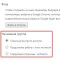 How to remove the start page in the Google Chrome browser
 The computer restarted unexpectedly or encountered an unexpected error