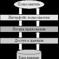
Sau synthesis methods. Synthesis of automatic control systems General procedure for the stage-by-stage synthesis of a linear automatic control system
Control questions for lecture 2
Ventilation systems. Ventilation systems are designed to ensure normal sanitary and hygienic conditions of the air environment in industrial premises. Depending on the performance of the functions, supply and exhaust systems, as well as air-thermal curtain systems.
Figure 5.11. Process unit automation diagram
Section 5. Lecture 2. Traditional methods of systems synthesis automatic control
Bespalov A.V., Kharitonov N.I. Control systems for chemical technological processes. - M .: ICC "Akademkniga, 2007. - 690 p.
Phillips Ch., Harbor R. Feedback control systems. - M .: LBZ, 2001 .-- 616 p.
Dorf R., Bishov R. Modern control systems. - M .: LBZ, 2002 .-- 832 p.
Besekersky V.A., Popov E.P. Theory of automatic control systems. - SPb: Profession, 2003 .-- 752 p.
Galperin M.V. Automatic control. - M .: FORUM: INFRA-M, 2004.-224 p.
Theory of automatic control / S.E. Dushin, N.S. Zotov, D.Kh. Imaev et al. - M .: Higher school, 2005. - 567 p.
Automatic control theory / V.N. Bryukhanov, M.G. Kosov, S.P. Protopopov and others - M. Higher School, 2000 .-- 268 p.
Bibliography
When is it justified to include a microprocessor system in a measuring system?
What does a microprocessor system solve as a part of measuring systems?
What is a microcontroller?
What is a microprocessor kit?
What is a microcomputer?
What is a microprocessor system?
8. What is the main task of supervisory management?
9. What is the main task of direct digital control?
3. Methods of classical and modern theory of automatic control. T.3. Methods of the modern theory of automatic control / Ed. N. D. Egupova. - M .: MVTU, 2000 .-- 748 p.
8. Ulyanov V.A., Leushin I.O., Gushchin V.N. Technological measurements, automation and control in technical systems. Part 1 - N. Novgorod: NSTU, 2000 .-- 336 p.
9.Ulyanov V.A., Leushin I.O., Gushchin V.N. Technological measurements, automation and control in technical systems. Part 2 - N. Novgorod: NSTU, 2002 .-- 417 p.
The synthesis of an ACS is understood as a directed calculation, with the ultimate goal of finding a rational structure of the system and establishing the optimal values of the parameters of its individual links. There are currently different points of view regarding the basis of synthesis.
Synthesis can be interpreted as an example of a variational problem and consider such a construction of the system, in which for given operating conditions (control and disturbing influences, interference, time constraints, etc.), a theoretical minimum of error is provided.
Synthesis can also be interpreted as an engineering problem, which is reduced to such a construction of the system, which ensures that the technical requirements for it are met. It is understood that of many possible solutions the engineer designing the system will select those that are optimal in terms of existing specific conditions and requirements for dimensions, weight, simplicity, reliability, etc.
Sometimes an even narrower meaning is put into the concept of engineering synthesis, a synthesis is considered with the aim of determining the type and parameters of corrective means that must be added to some unchanged part of the system (an object with a control device) in order to provide the required dynamic properties.
In the engineering synthesis of ACS, it is necessary to ensure, firstly, the required accuracy and, secondly, the acceptable nature of the transient processes.
The solution of the first problem in most cases comes down to determining the required transmission coefficient of an open-loop system, and, if necessary, the type of corrective means that increase the accuracy of the system (combined control, isodromic mechanisms, etc.) This problem can be solved by determining errors in typical modes based on accuracy criteria.
The solution of the second problem - ensuring acceptable transient processes - is almost always more difficult due to the large number of variable parameters and the ambiguity of the solution to the problem of damping the system.
Root method. There is a characteristic equation of the system
From the point of view of the fastest decay of the transient process, it is important that the real parts of the roots of the characteristic equation are largest. The sum of the real parts of all roots is numerically equal to the first coefficient of the characteristic equation. Therefore, for a given value of this coefficient, the most advantageous results are obtained when the real parts of all roots are equal, but this is not realistic. Calculations show that from the total number of roots of the characteristic equation, always select two or three roots with a smaller real part in absolute value, which determine the course of the main process. The rest of the roots characterize rapidly decaying components that affect only the initial stage of the transient process.
It is convenient to represent the previous equation in the form
The second factor will determine the basic nature of the process. To reduce the errors of the designed system, it is important that the coefficient in the main multiplier is as large as possible. However, an excessive increase leads to an oscillatory nature of the transient. The optimal ratio between the coefficients and is determined from the condition for obtaining the damping in one period ξ = 98%, which corresponds to the expression, where are the real and imaginary parts of the complex root characterizing the main process. From here you can get.
The factor that determines the relationship between the coefficients of the main factor of the characterizing equation is a criterion for the transient mode, depending on the chosen degree of attenuation.
The synthesis of the control system begins with the fact that the characteristic equation is found for the selected structural scheme and the introduction of corrective means. Then the parameters of the main channel and the correcting means are varied in such a way as to obtain the required value of the coefficients of the characteristic equation.
This method turns out to be quite effective in the case of a relatively low degree of the characteristic equation (= 2-4). The disadvantage of this method is that it is necessary to specify the type of corrective agents.
Root locus method. The quality of the control system in terms of speed and stability margin can be characterized by the location of the roots of the numerator and denominator transfer function closed system, i.e. the location of the zeros and poles of the transfer function.
Knowing these roots, you can avoid their location on the complex plane of the roots. When calculating the system, it is advisable to trace how the general picture of the location of the roots changes when individual parameters are changed, for example, the transmission coefficient of an open-loop system, time constants of correcting circuits, etc., in order to establish the optimal values of these parameters.
With a smooth change in the value of any parameter, the roots will alternate on the plane of the roots, tracing a certain curve, which we will call root hodograph or the trajectory of the roots. Having built the trajectories of all the roots, you can choose such a value of the variable parameter that corresponds to the best location of the roots.
In this case, the calculation of the roots can be performed using standard programs for digital machines with the output of the trajectory of the roots on the display screen.
Standard transient response method. To obtain the required values of the coefficients of the transfer function of an open-loop system, you can use the standard transient characteristics. For greater generality, these characteristics are constructed in a normalized form. In this case, relative time is plotted along the time axis, where is the geometric mean root of the characteristic equation, which determines the speed of the system.
When constructing standard transient characteristics, it is necessary to specify a certain distribution of the roots of the characteristic equation.
Method of logarithmic amplitude characteristics. The most acceptable for synthesis purposes are logarithmic amplitude characteristics, since the construction of the LAH, as a rule, can be done almost without computing work... It is especially convenient to use asymptotic LACs.
The synthesis process usually includes the following operations:
o building the desired LAH;
o construction of a disposable LAH;
o determination of the type and parameters of the correcting device;
o technical implementation of corrective devices;
o verification calculation and construction of the transient process.
The synthesis is based on the following quality indicators:
¨ overshoot with a single step action at the input;
¨ transient time;
¨ error rates.
Synthesis of ACS by the method of logarithmic amplitude characteristics is currently one of the most convenient and intuitive. The most difficult point in the calculation by the method of logarithmic amplitude characteristics is to establish a connection between the quality indicators of the transient process and the parameters of the desired LAH, which is explained by the relatively complex relationship between the transient linear system and its frequency properties. characteristic to pass to the quality assessment directly according to its frequency properties.
Synthesis of ACS based on frequency quality criteria. To assess the quality of any control system, including the tracking system, it is necessary to know its accuracy, characterized by errors in some typical modes, performance, determined by the ability of the system to operate at high speeds and accelerations of the input action or by the speed of transient processes, and the stability margin , showing the tendency of the system to oscillate. In accordance with this, we can talk about accuracy criteria, performance criteria and stability margin criteria. When using frequency criteria, it is necessary to rely on certain frequency properties of the system.
When evaluating the accuracy by errors when reproducing the harmonic input action, it is possible to simultaneously evaluate and the performance merge into one criterion of the dynamic accuracy of the control system. The error of the follower system is not understood as an actual mismatch between the master and slave axes, but only the mismatch signal detected by the sensitive element.
Hardware synthesis of automatic and automated control systems traditional methods includes the following set of tools: sensors, converters, masters, regulators, amplifiers, actuators and regulating bodies.
In the economy of workshops with heating and melting units, various types of boilers are often used for heat recovery. Boiler safety and compliance with technical supervision requirements are carried out by solving the following tasks:
· Automatic blocking draining water from the boiler when the liquid level and water pressure drop to the permissible limit;
· Duplication of control of the water level in the boiler using reliable automation equipment;
The use of control equipment, which allows, if necessary, to switch to manual remote control unit;
Emergency supply sound signal when the shut-off valve is triggered;
· Light signaling of deviations from the norm of individual monitored values.
Automatic regulation of the water level in the proposed ACS is carried out using modern equipment of the "Kontur - 2" complex, manufactured by JSC "MZTA" (Moscow).
For automatic control of pressure and level, measuring transducers of the "Sapphire -22 M" type of various modifications and two-channel secondary devices of the TRMO-PIC type of the "Euro" series, produced by the "OWEN" company (Moscow), were used. Such devices can work with sensors of unified electrical signals, are equipped with digital indicators and have built-in power supplies for measuring transducers.
The use of the eight-channel AC2 network adapter allows the pairing of devices of the TRMO-PIC type with a serial COM - port of an IBM - compatible computer. To transmit information signals, the RS-232 communication interface is used (Fig. 5.11).
The specification of the used automation tools is given in table. 5.1.
Serious attention has been recently paid to the automation of hot water boilers, heating points and district heating systems. Without this, uninterrupted and high-quality heat supply to industrial enterprises and consumers of the housing and communal sector is impossible.
Table 5.1 Specification of the used equipment
The LFC method is one of the most common methods for the synthesis of automatic control, since the LFC construction, as a rule, can be performed with practically no computational work. It is especially convenient to use asymptotic “ideal” LFC.
The synthesis process usually includes the following operations;
1. Construction of the LAFC of the unchangeable part of the system.
The immutable part of the control system contains the control object and the executive element, as well as the main feedback element and the comparison element of the LAFC of the unchangeable part are built according to the transfer function of the open-loop unchangeable part of the system.
2. Building the desired part of the LACHH.
The schedule of the desired LAFC is made on the basis of those requirements that are imposed on the projected control system. The desired LFCH Lzh can be conditionally divided into three parts: low-frequency, mid-frequency and high-frequency.
2.1 The low-frequency part is determined by the static accuracy of the system, the accuracy in steady-state conditions. In a static system, the low-frequency asymptote is parallel to the abscissa axis. In an astatic system, the slope of this asymptote is –20 mdB / dec, where is the order of astatism (= 1.2). The ordinate of the low-frequency part Lzh is determined by the value of the transfer coefficient K of the open-loop system. The wider the low-frequency part Lzh, the more high frequencies reproduced by the system without closed attenuation.
2.2 The mid-frequency part is the most important, since it determines stability, stability margin and, consequently, the quality of transients, usually assessed by quality indicators transient response... The main parameters of the mid-frequency asymptote are its slope and cutoff frequency cp (the frequency at which Lzh crosses the abscissa axis). The greater the slope of the mid-frequency asymptote, the more difficult it is to ensure good dynamic properties of the system. Therefore, the most reasonable slope is -20dB / dec and very rarely it exceeds -40dB / dec. The cutoff frequency cp determines the system speed and the value of the overshoot value. The more cp, the higher the speed, the less time regulation TPP transient response, the greater the overshoot.
2.3 The high-frequency part of the LAFC insignificantly affects the dynamic properties of the system. It is better to have the slope of its asymptote as large as possible, which reduces the required power of the actuator and the effect of high-frequency interference. Sometimes, when calculating, the high-frequency LFC is not taken into account.

where is the coefficient depending on the overshoot value,
Should be selected according to the schedule shown in Figure 1.

Figure 18- Graph for determining the permissible overshoot of the coefficient.
The ordinate of the low-frequency asymptote is determined accordingly by the coefficient
The gain and slope of the high frequency asymptote of the transient open CAP.
3. Determination of the parameters of the correcting device.
3.1 The LAFC graph of the correcting device is obtained by subtracting the unchanged values of the graph from the value of the graph of the desired LAFC, after which its transfer function is determined from the LAFC of the correcting device.
3.2 According to the transfer function of the regulator, the electrical circuit for the implementation of the correcting device and the values of its parameters are calculated. The regulator circuit can be on passive or active elements.
3.3 The transfer function of the correcting device, obtained in paragraph 3.1, is included in the generalized block diagram of the ACS.
Example:
6. Synthesis of an automatic control system by the method of logarithmic frequency characteristics.
The task of the correction is to improve the accuracy of systems both in steady-state and transient modes. It arises when the desire to reduce control errors in typical modes leads to the need to use such values of the gain of an open-loop ACS, at which, without taking special measures (installing additional links - correcting devices), the system turns out to be unstable.
| Types of corrective devices |
There are three types of main correcting devices (Figure 6.1): serial (W k1 (p)), in the form of local feedback (W k2 (p)) and parallel (W k3 (p)).

Figure 6.1. Structural diagrams corrective devices.
The correction method using sequential correcting devices is simple in calculations and technically easy to implement. Therefore, it has found wide application, especially when correcting systems that use electrical circuits with an unmodulated signal. Sequential correcting devices are recommended to be used in systems in which there is no drift of the link parameters. Otherwise, adjustment of the correction parameters is required.
Correction of control systems using a parallel correcting device is effective when there is a need for high-frequency shunting of inertial links. In this case, rather complex control laws are formed with the introduction of derivatives and integrals of the error signal with all the resulting disadvantages.
Correction by local (local) feedback is used most often in automatic control systems. The advantage of correction in the form of local feedback is a significant weakening of the influence of nonlinearities of the characteristics of the links included in the local loop, as well as a decrease in the dependence of the control parameters on the drift of device parameters.
The use of one or another type of corrective device, i.e. sequential links, parallel links or feedbacks, is determined by the convenience of technical implementation. In this case, the transfer function of the open-loop system must be the same with different switching on of the correcting links:
The above formula (6.1) makes it possible to recalculate one type of correction for another in order to choose the most simple and easy to implement.
Department of Distance and Correspondence
| ACS synthesis |
System synthesis is a directed calculation, the purpose of which is: building a rational structure of the system; finding the optimal values of the parameters of individual links. With many possible solutions, it is first necessary to formulate the technical requirements for the system. And under the condition of certain restrictions imposed on the ACS, it is necessary to select an optimization criterion - static and dynamic accuracy, speed, reliability, energy consumption, price, etc.
In engineering synthesis, the following tasks are set: achieving the required accuracy; ensuring a certain nature of transient processes. In this case, the synthesis is reduced to the definition of the type and parameters of the corrective means that must be added to the unchangeable part of the system in order to ensure the quality indicators are not worse than the specified ones.
The most widespread in engineering practice is the frequency synthesis method using logarithmic frequency characteristics.
The control system synthesis process includes the following operations:
- construction of the available LAFC L 0 (ω) of the original system W 0 (ω), consisting of a controlled object without a regulator and without a correcting device;
- construction of the low-frequency part of the desired LAFC based on the requirements for accuracy (astatism);
- construction of a mid-frequency section of the desired LAFC, providing a given overshoot and control time t p ACS;
- matching the low- with the mid-frequency section of the desired L and H. provided that the simplest corrective device is obtained;
- Refinement of the high-frequency part of the desired L.A.kh. based on the requirements for ensuring the required stability margin;
- determination of the type and parameters of the sequential correcting device L ku (ω) = L w (ω) - L 0 (ω), since W w (p) = W ku (p) * W 0 (p);
- technical implementation of corrective devices. If necessary, recalculation is carried out for an equivalent parallel link or OS;
- verification calculation and construction of the transient process.
Construction of the desired L.A.Kh. produced in parts.
The low-frequency part of the desired L.A.kh. is formed from the condition of ensuring the required accuracy of the control system in the steady state, that is, from the condition that the steady-state error of the system Δ () should not exceed the specified value Δ () ≤Δ h.
Formation of a forbidden low-frequency region for the desired LAH. Maybe different ways... For example, when applying a sinusoidal signal to the input, it is required to ensure the following permissible indicators: Δ m - the maximum amplitude of the error; v m - maximum speed tracking; ε m - maximum acceleration of tracking. Earlier it was shown that the amplitude of the error when reproducing a harmonic signal Δ m = g m / W (jω k), i.e. is determined by the modulus of the transfer function of the open ACS and the amplitude of the input action g m. In order for the ACS error not to exceed Δ s, the desired l.h. must pass at least control point A to with coordinates: ω = ω to, L (ω to) = 20lg | W (jω k) | = 20lg g m / Δ m.
The relations are known:
g (t) = g m sin (ω k t); g "(t) = g m (ω k t); g" "(t) = -g m ω k 2 sin (ω k t);
v m = g m k; ε m = g m ω k 2; g m = v m 2 / ε m; ω k = ε m / v m. (6.2)
The forbidden region corresponding to a system with 1st order astatism and ensuring operation with the required error in tracking amplitude, tracking speed and acceleration is shown in Fig. 6.2.

Figure 6.2. The forbidden area of the desired l.a.kh.
Quality factor for speed K ν = v m / Δ m, quality factor for acceleration K ε = ε m / Δ m. In the event that it is required to provide only a static control error when the signal g (t) = g 0 = const is applied to the input, then the low-frequency section of the desired L.A.h. should have a slope of 0 dB / dec and pass at the level of 20logK tr, where K tr (the required gain of an open-loop ACS) is calculated by the formula
Δ z () = ε st = g 0 / (1+ K tr), whence K tr ≥ -1.
If it is required to provide tracking with a given accuracy from the reference action g (t) = νt at ν = const, then the steady-state speed error ε ck () = ν / K tr. From here, K tr = ν / ε cc is found and the low-frequency part of the desired LAX is carried out with a slope of -20 dB / dec through the speed Q factor K ν = K tr = ν / ε cc or a point with coordinates: ω = 1 s -1, L ( 1) = 20lgk tr dB.
As it was shown earlier, the mid-frequency section of the desired l.c.h. provides the main indicators of the quality of the transient process - overshoot σ and regulation time tp. should have a slope of -20 dB / dec and cross the frequency axis at the cutoff frequency ω cf, which is determined by the nomograms of V.V. Solodovnikov (Fig. 6.3). It is recommended to take into account the astatism order of the designed system and choose ω cf according to the corresponding nomogram.

Figure 6.3. Solodovnikov quality nomograms:
a - for astatic ACS of the 1st order; b - for static ACS
For example, for σ m = 35% and t p = 0.6 s, using the nomogram (Fig. 6.3, a) for an astatic system of the 1st order, we obtain t p = 4.33 π / ω avg or ω avg = 21.7 s -1 ...
Through ω cf = 21.7 s -1, it is necessary to draw a straight line with a slope of -20 dB / dec, and the width of the mid-frequency section is determined from the condition of ensuring the required stability margin in modulus and phase. Known different approaches to the establishment of stability margins. It must be remembered that the higher the cutoff frequency in the system, the greater the likelihood that the calculations will be affected by the error of the small time constants of individual ACS devices that are not taken into account. Therefore, it is recommended to artificially increase the phase and modulus stability margins with an increase in ω cf. So for two types of ACS it is recommended to use the table given in the table. With high quality requirements for transients, for example,
20%<σ m <24%;  ,
,
25%<σ m <45%;  ,
,
the following average stability indicators are recommended: φ zap = 30 °, H m = 12 dB, -H m = 10 dB.
Figure 6.4 shows a view of the mid-frequency section of the desired LH, the width of which provides the required stability margins.

Figure 6.4. The mid-frequency part of the desired l.c.h.
After that, the sections of middle and low frequencies are matched by straight segments with slopes of -40 or -60 dB / dec from the condition of obtaining the simplest correcting device.
The slope of the high-frequency section of the desired l.h. it is recommended to leave equal to the slope of the high-frequency section of the available LAH. In this case, the correcting device will be more immune to interference. Coordination of the mid- and high-frequency sections of the desired LAH. is also carried out taking into account obtaining a simple corrective device and, in addition, ensuring the necessary stability margins.
The transfer function of the desired open-loop system W w (p) is found by the form of the desired l.h. L w (ω). Then the phase frequency response of the desired open-loop control system and the transient response of the desired closed-loop system are constructed, and the actually obtained quality indicators of the designed system are estimated. If they satisfy the required values, then the construction of the desired l.h. is considered complete, otherwise the constructed desired LFCs must be adjusted. To reduce overshoot, the mid-frequency section of the desired LH is expanded. (increase the value ± H m). To improve system performance, it is necessary to increase the cutoff frequency.
To determine the parameters of a sequential correcting device, it is necessary:
a) subtract from the desired L. and x. L w available l and h. L 0, i.e. find l.h. minimum-phase correcting device L ku;
b) by type of L. and x. sequential correcting device L ku write its transfer function and, using the reference literature, select a specific circuit and implementation.
Figure 6.5 shows an example of determining the transfer function of a serial correcting device.

Figure 6.5. LAH available L 0, desired L w open-loop system
and a sequential correcting device L ku
After graphic subtraction, we obtain the following transfer function of the correcting device

A parallel correcting device or a correcting device in the form of local feedback can be obtained by recalculation according to formula (6.1).
Based on the obtained transfer function W ku (p), it is necessary to design a real correcting device, which can be implemented in hardware or software. In the case of hardware implementation, it is required to select the circuit and parameters of the correcting link. In the literature, there are tables of typical correcting devices, both passive and active, both in direct and alternating current. In the event that it is used to control the ACS of a computer, then software implementation is preferable.
Original Russian Text © V.N. Bakaev, Vologda 2004. Development of the electronic version: M.A. Gladyshev, I.А. Churanov.
Vologda State Technical University.
Department of Distance and Distance Learning
Systems built on the principle of subordinate regulation, which is illustrated in Figure 6.6, are now widely used. The system provides n control loops with their own controllers W pi (p), and the output signal of the external loop controller is the prescribed value for the internal loop, i.e. the work of each inner loop is subordinate to the outer loop.

Figure 6.6. Structural diagram of the ACS of subordinate regulation
Two main advantages determine the operation of subordinate control systems.
1. Simplicity of calculation and setting. The adjustment during the commissioning process is carried out starting from the inner contour. Each circuit includes a regulator, due to the parameters and structure of which standard characteristics are obtained. Moreover, in each circuit, the largest time constant is compensated.
2. Convenience of limiting the limiting values of the intermediate coordinates of the system. This is achieved by limiting the output of the external loop controller to a certain value.
At the same time, it is obvious from the principle of constructing a subordinate control system that the speed of each outer loop will be lower than the speed of the corresponding inner loop. Indeed, if in the first loop the cutoff frequency of the l.c.h. will be 1 / 2T μ, where 2T μ is the sum of small uncompensated time constants, then even in the absence of other links with small time constants in the external loop, the cutoff frequency of its l.c.h. will be 1 / 4T μ, etc. Therefore, slave control systems are rarely built with more than three loops.
Take a typical circuit in Figure 6.7 and tune it to modular (MO) and symmetric (CO) optima.

Figure 6.7. Typical circuit diagram
The diagram in Fig.6.7 indicates: T μ - the sum of small time constants;
T about - large time constant to be compensated; K ε and K O - respectively, the gains of blocks with small time constants and the control object. It should be noted that the type of controller W p (p) depends on the type of link, the time constant of which should be compensated. It can be P, I, PI and PID. Take a PI controller as an example:
![]() .
.
For the modular optimum, select the parameters:
![]()
Then the transfer function of the open loop will have the form:
![]()
The logarithmic frequency characteristics corresponding to the transfer function W (p) are shown in Figure 6.8, a.

Figure 6.8. LFC and h (t) with modular tuning
With a stepped control action, the output value for the first time reaches a steady-state value after a time of 4.7Tμ, the overshoot is 4.3%, and the phase margin is 63 ° (Figure 6.8, b). The transfer function of the closed ACS has the form

If we represent the characteristic equation of a closed ACS in the form of T 2 p 2 + 2ξ Tr + 1 = 0, then the damping coefficient at the modular optimum has the value ![]() ... At the same time, it can be seen that the regulation time does not depend on the large time constant T about. The system has first order astatism. When tuning the system to a symmetric optimum, the parameters of the PI controller are selected as follows:
... At the same time, it can be seen that the regulation time does not depend on the large time constant T about. The system has first order astatism. When tuning the system to a symmetric optimum, the parameters of the PI controller are selected as follows:
![]()
Then the transfer function of the open loop has the form


The corresponding logarithmic frequency characteristics and the transient process graph are shown in Figure 6.9.

Figure 6.9. LFC and h (t) when tuning to a symmetric optimum
The time for the first achievement of the steady-state value by the output value is 3.1T μ, the maximum overshoot reaches 43%, the phase margin is -37 °. ACS acquires second order astatism. It should be noted that if the link with the longest time constant is aperiodic of the 1st order, then with the PI - controller at T o = 4T μ, the transient processes correspond to the processes when tuned to the MO. If T about<4Т μ , то настройка регулятора на τ=Т μ теряет смысл. Необходимо выбрать другой тип регулятора.
In TAU, other types of optimal regulator settings are also known, for example:
- binomial, when the characteristic equation of the automatic control system is represented in the form (p + ω 0) n - where ω 0 is the modulus of an n - multiple root;
- butterworth, when the characteristic equations of the automatic control system of various orders have the form 
It is advisable to use these settings when the system uses modal control for each coordinate.
Original Russian Text © V.N. Bakaev, Vologda 2004. Development of the electronic version: M.A. Gladyshev, I.А. Churanov.
Vologda State Technical University.
| Construction of the transient process |
There are three groups of methods for constructing transient processes: analytical; graphic, using frequency and transient characteristics; construction of transient processes using a computer. In the most difficult cases, computers are used, which allow, in addition to modeling the ACS, to connect individual parts of the real system to the machine, i.e. close to the experimental method. The first two groups are used mainly in the case of simple systems, as well as at the stage of preliminary research with a significant simplification of the system.
Analytical methods are based on solving the differential equations of the system or determining the inverse Laplace transform of the transfer function of the system.
Calculation of transient processes by frequency characteristics is used when the analysis of the ACS from the very beginning is carried out by frequency methods. In engineering practice, the method of trapezoidal frequency characteristics developed by V.V. Solodovnikov has become widespread for assessing quality indicators and constructing transient processes in automatic control systems.
It has been established that if the system is acted upon by a single setting action, i.e. g (t) = 1 (t), and the initial conditions are zero, then the response of the system, which is a transient characteristic, in this case can be defined as
 (6.3)
(6.3)
 (6.4)
(6.4)
where P (ω) is the real frequency response of the closed-loop system; Q (ω) is the imaginary frequency response of a closed-loop system, i.e. Ф g (jω) = P (ω) + jQ (ω).
The construction method consists in the fact that the constructed real characteristic P (ω) is divided into a series of trapezoids, replacing approximately curved lines with rectilinear segments so that when all the ordinates of the trapezoids are added together, the original characteristic of Fig. 6.10 is obtained.

Figure 6.10. The material characteristic of a closed system
where: ω pi and ω cfi are the frequency of uniform transmission and the cutoff frequency of each trapezoid, respectively.
Then, for each trapezoid, the slope coefficient ω pi / ω avg is determined, and the transient processes from each trapezoid hi are constructed from the table of h-functions. Dimensionless time τ is given in the table of h-functions. To obtain real time t i, it is necessary to divide τ by the cutoff frequency of the given trapezoid. The transient process for each trapezoid must be increased by P i (0) times, since in the table of h-functions, transient processes from single trapezoids are given. The transient process of the ACS is obtained by the algebraic summation of the constructed h i processes from all trapezoids.
Original Russian Text © V.N. Bakaev, Vologda 2004. Development of the electronic version: M.A. Gladyshev, I.А. Churanov.
Vologda State Technical University.
Department of Distance and Distance Learning
| Questions on topic number 6 |
1. What is meant by improving the quality of the management process and how is this achieved?
2. Name the linear standard control law.
3. Tell us about typical control laws and typical regulators.
4. What is the purpose of corrective devices? Indicate how they are included and what is specific.
5. Explain the formulation of the problem of systems synthesis.
6. List the stages of systems synthesis.
7. Explain the construction of the desired LAH of the designed system.
8. How is the transfer function of the open-loop projected system formed?
9. How are the transfer functions of the correcting devices determined?
10. What are the advantages and disadvantages of parallel and series correcting devices?
11. How are "closure" nomograms used?
12. List the methods for constructing transient processes.
13. How to determine the steady-state value of the transient process by the material characteristic?
14.How to change the desired l.a.kh. to increase the stability margins?
Original Russian Text © V.N. Bakaev, Vologda 2004. Development of the electronic version: M.A. Gladyshev, I.А. Churanov.
Vologda State Technical University.
Department of Distance and Distance Learning
Topic number 7: Non-linear self-propelled guns
| Introduction |
Most of the characteristics of real devices are generally nonlinear and some of them cannot be linearized, since have discontinuities of the second kind and the piecewise linear approximation is inapplicable to them. The operation of real links (devices) can be accompanied by such phenomena as saturation, hysteresis, backlash, the presence of a dead zone, etc. Nonlinearities can be natural or artificial (intentionally introduced). Natural nonlinearities are inherent in systems due to the nonlinear manifestation of physical processes and properties in individual devices. For example, the mechanical characteristic of an induction motor. Artificial nonlinearities are introduced by developers into systems to ensure the required quality of work: for systems that are optimal in terms of speed, relay control is used, the presence of nonlinear laws in search and non-search extreme systems, systems with variable structure, etc.
Non-linear system such a system is called, which includes at least one element, the linearization of which is impossible without losing the essential properties of the control system as a whole. The essential signs of nonlinearity are: if some coordinates or their time derivatives are included in the equation in the form of products or a degree different from the first; if the coefficients of the equation are functions of some coordinates or their derivatives. When composing differential equations for nonlinear systems, differential equations are first compiled for each device in the system. In this case, the characteristics of devices that can be linearized are linearized. Elements that do not allow linearization are called substantially nonlinear... The result is a system of differential equations in which one or more equations are nonlinear. Devices that can be linearized form the linear part of the system, and devices that cannot be linearized form the non-linear part. In the simplest case, the block diagram of an ACS of a nonlinear system is a series connection of an inertialess nonlinear element and a linear part, covered by feedback (Figure 7.1). Since the principle of superposition is not applicable to nonlinear systems, then, when carrying out structural transformations of nonlinear systems, the only restriction in comparison with structural transformations of linear systems is that it is impossible to transfer nonlinear elements through linear ones and vice versa.

Rice. 7.1. Functional diagram of a nonlinear system:
NE - non-linear element; LCH - linear part; Z (t) and X (t)
the output and input of the nonlinear element, respectively.
Classification of nonlinear links is possible according to various criteria. The most widespread classification is based on static and dynamic characteristics. The former are represented as nonlinear static characteristics, and the latter as nonlinear differential equations. Examples of such characteristics are given in. Figure 7.2. examples of unambiguous (without memory) and multivalued (with memory) nonlinear characteristics are given. In this case, the direction (sign) of the signal speed at the input is taken into account.

Figure 7.2. Static characteristics of nonlinear elements
The behavior of nonlinear systems in the presence of significant nonlinearities has a number of features that differ from the behavior of linear ACS:
1.
the output value of a nonlinear system is disproportionate to the input action, i.e. the parameters of nonlinear links depend on the magnitude of the input action;
2.
transients in nonlinear systems depend on the initial conditions (deviations). In this regard, the concepts of stability "in small", "in large", "in general" are introduced for nonlinear systems. A system is stable "in small" if it is stable for small (infinitesimal) initial deviations. A system is stable "in the large" if it is stable at large (finite in magnitude) initial deviations. The system is stable "as a whole" if it is stable at any large (unlimited in magnitude) initial deviations. Figure 7.3 shows the phase trajectories of the systems: stable "in the whole" (a) and systems stable "in the big" and unstable "in the small" (b);

Figure 7.3. Phase trajectories of nonlinear systems
3.
nonlinear systems are characterized by a mode of continuous periodic oscillations with constant amplitude and frequency (self-oscillations), which occurs in systems in the absence of periodic external influences;
4.
with damped oscillations of the transient process in nonlinear systems, a change in the oscillation period is possible.
These features have led to the lack of common approaches in the analysis and synthesis of nonlinear systems. The developed methods make it possible to solve only local nonlinear problems. All engineering methods for studying nonlinear systems are divided into two main groups: exact and approximate. The exact methods include the method of A.M. Lyapunov, the method of the phase plane, the method of point transformations, the frequency method of V.M. Popov. Approximate methods are based on the linearization of nonlinear equations of the system using harmonic or statistical linearization. The limits of applicability of this or that method will be discussed below. It should be noted that in the foreseeable future there is a need for further development of the theory and practice of nonlinear systems.
A powerful and effective method for studying nonlinear systems is modeling, the toolkit of which is a computer. At present, many theoretical and practical problems that are difficult for analytical solution can be relatively easily solved with the help of computer technology.
The main parameters characterizing the operation of nonlinear ACS are:
1.
The presence or absence of self-oscillations. If there are self-oscillations, then it is necessary to determine their amplitude and frequency.
2.
Time for the controlled parameter to reach the stabilization mode (response speed).
3.
The presence or absence of a sliding mode.
4.
Determination of special points and special trajectories of movement.
This is not a complete list of the studied indicators that accompany the operation of nonlinear systems. Systems are extreme, self-adjusting, with variable parameters, and require evaluation and additional properties.
Original Russian Text © V.N. Bakaev, Vologda 2004. Development of the electronic version: M.A. Gladyshev, I.А. Churanov.
Vologda State Technical University.
Department of Distance and Distance Learning.
The idea of the harmonic linearization method belongs to N.M. Krylov and N.N. Bogolyubov and is based on replacing the nonlinear element of the system with a linear link, the parameters of which are determined under a harmonic input action from the condition of equality of the amplitudes of the first harmonics at the output of the nonlinear element and its equivalent linear link. The method is approximate and can be used only when the linear part of the system is a low-pass filter, i.e. filters out all harmonic components arising at the output of the nonlinear element, except for the first harmonic. In this case, the linear part can be described by a differential equation of any order, and the nonlinear element can be both single-valued and multivalued.
The method of harmonic linearization (harmonic balance) is based on the assumption that a harmonic action with frequency ω and amplitude A is applied to the input of a nonlinear element, i.e. x = A sinωt. Assuming that the linear part is a low-pass filter, the spectrum of the output signal of the linear part is limited only by the first harmonic determined by the Fourier series (this is the approximation of the method, since higher harmonics are discarded from consideration). Then the relationship between the first harmonic of the output signal and the input harmonic action of the nonlinear element is represented as a transfer function:
![]() (7.1)
(7.1)
Equation (7.1) is called the harmonic linearization equation, and the coefficients q and q "are the harmonic linearization coefficients, depending on the amplitude A and the frequency ω of the input. For various types of nonlinear characteristics, the harmonic linearization coefficients are summarized in the table. It should be noted that for static single-valued coefficients q "(A) = 0. Subjecting equation (7.1) to the Laplace transformation under zero initial conditions with the subsequent replacement of the operator p by jω (p = jω), we obtain the equivalent complex transfer coefficient of the nonlinear element
W ne (jω, A) = q + jq ". (7.2)
After the harmonic linearization has been carried out, for the analysis and synthesis of nonlinear ACS, it is possible to use all the methods used to study linear systems, including the use of various stability criteria. When studying nonlinear systems based on the method of harmonic linearization, first of all, the question of the existence and stability of periodic (self-oscillatory) modes is solved. If the periodic regime is stable, then in the system there are self-oscillations with a frequency ω 0 and an amplitude A 0. Consider a nonlinear system that includes a linear part with a transfer function
 (7.3)
(7.3)
and a non-linear element with an equivalent complex gain (7.2). The design block diagram of a nonlinear system takes the form of Figure 7.5.

Figure 7.5. Block diagram of a nonlinear ACS
To assess the possibility of the occurrence of self-oscillations in a nonlinear system by the method of harmonic linearization, it is necessary to find the conditions of the stability boundary, as was done in the analysis of the stability of linear systems. If the linear part is described by the transfer function (7.3), and the nonlinear element (7.2), then the characteristic equation of the closed-loop system will have the form
d (p) + k (p) (q (ω, A) + q "(ω, A)) = 0 (7.4)
Based on the Mikhailov stability criterion, the stability boundary will be the passage of the Mikhailov hodograph through the origin. From expressions (7.4), it is possible to find the dependence of the amplitude and frequency of self-oscillations on the parameters of the system, for example, on the transfer coefficient k of the linear part of the system. For this, it is necessary to consider the transfer coefficient k as a variable in equations (7.4), i.e. write this equation in the form:
d (jω) + K (jω) (q (ω, A) + q "(ω, A)) = Re (ω 0, A 0, K) + Jm (ω 0, A 0, k) = 0 (7.5)
where ω o and A o are the possible frequency and amplitude of self-oscillations.
Then, equating to zero the real and imaginary parts of equation (7.5)
 (7.6)
(7.6)
The method of logarithmic frequency characteristics is used to determine the frequency transfer functions of correcting devices that bring the dynamic performance closer to the desired one. This method is most effectively used to synthesize systems with linear or digital correcting devices, since in such systems the frequency characteristics of the links do not depend on the amplitude of the input signals. Synthesis of ACS by the method of logarithmic frequency characteristics includes the following operations:
At the first stage, according to the known transfer function of the unchangeable part of the ACS, its logarithmic frequency characteristic is constructed. In most cases, the use of asymptotic frequency characteristics is sufficient.
At the second stage, the desired logarithmic frequency response of the ACS is constructed, which would satisfy the set requirements. Determination of the type of the desired LAFC is carried out based on the purpose of the system, the time of the transient process, overshoot and error rates. In this case, typical frequency characteristics are often used for systems with different orders of astatism. When constructing the desired LAFC, it is necessary to be sure that the form of the amplitude characteristic completely determines the nature of the transient processes, and there is no need to introduce the phase frequency response into consideration. The latter is true in the case of minimum-phase systems, which are characterized by the absence of zeros and poles located in the right half-plane. When choosing the desired logarithmic amplitude and phase characteristics, it is important that the latter provides the required stability margin at the system cutoff frequency. For this, special nomograms are used, the form of which is shown in Fig. 1.
Figure 16-1 Curves for choosing the stability margin in amplitude (a) and phase (b) depending on the amount of overshoot
Satisfactory quality indicators of the ACS in dynamic modes are achieved when the amplitude characteristic of the abscissa axis crosses the slope of –20 dB / dec.
Figure 16-2 Determination of the characteristics of the PKU
At the last stage, the frequency properties of the correcting device are determined by comparing the frequency characteristics of the uncorrected system and the desired frequency characteristics. When using linear correction means, the logarithmic frequency response of the sequential correcting device (SCU) can be found by subtracting the LAFC of the uncorrected system from the desired LAFC of the ACS, that is
Hence
It should be noted that it is easy to determine the transfer functions of the links in the direct or feedback circuit using the transfer function of the sequential correcting device, with the help of which the dynamic indicators of the ACS are corrected.
The next step is to determine the implementation method, circuit and parameters of the correcting device.
The last stage in the synthesis of the correction device is the verification calculation of the ACS, which consists in the construction of graphs of transient processes for the system with the selected correction device. At this stage, it is advisable to use computer technology and modeling software systems VinSim, WorkBench, CircuitMaker, MathCAD.
Send your good work in the knowledge base is simple. Use the form below
Students, graduate students, young scientists who use the knowledge base in their studies and work will be very grateful to you.
Posted on http://www.allbest.ru//
Posted on http://www.allbest.ru//
Ministry of Education and Science of the Russian Federation
FGBOU VO Ivanovo State Chemical-Technological University of Technical Cybernetics and Automation.
COURSE WORK
By discipline: Theory of automatic control
Topic: Synthesis of automatic control systems
Ivanovo 2016
Transient function of the control object
Table 1. Transient function of the control object.
annotation
In this course work, the object of research is a stationary inertial object with a delay, represented by a transition function, as well as a control system for it.
The research methods are elements of the theory of automatic control, mathematical and simulation modeling.
With the help of identification methods, approximation and a graphical method, models of objects in the form of transfer functions were obtained, a model was established that most accurately describes a given object.
After choosing the model of the object, the calculations of the controller tuning parameters were performed using the Ziegler-Nichols methods and extended frequency characteristics.
To determine the method by which the best settings for the controller of the closed-loop automatic control system were found, it was simulated in the Matlab environment using the Simulink package. Based on the simulation results, a method was selected, with the help of which the regulator settings were calculated that best meet the specified quality criterion.
The synthesis of a control system for a multidimensional object was also made: a cascade control system, a combined control system, an autonomous control system. The parameters of adjusting PI-regulators, compensators were calculated, responses to typical influences were obtained.
List of keywords:
Control object, controller, settings, control system.
Volume Details:
Amount of work- pages
Number of tables
Number of illustrations - 32
Number of sources used - 3
Introduction
In this course work, the initial data is the transient function of the control object along one of the dynamic channels. It is necessary to carry out parametric identification of the object specified by the transition function by the graphical method, by methods of approximation and identification.
Based on the data obtained, we establish which model more accurately describes the given object. The solution to this problem is a rather urgent problem, since often we have not the mathematical model itself, but only its acceleration curve.
After choosing the model of the object, we calculate the parameters of the PI controller. The calculation is carried out using the Ziegler-Nichols methods and extended frequency characteristics. In order to determine by which method the best settings of the regulator were found, we use the degree of process damping as a quality criterion.
In this work, the synthesis of a control system for a multidimensional object of three types is carried out: autonomous, cascade, combined. The parameters for adjusting the regulators were calculated, the responses of the system through various channels to typical influences were investigated.
This course work is educational. The skills gained in the course of its implementation can be used in the course of the coursework on modeling management systems and the final qualification work.
1.Object identification
1.1 Identification using the System Identification ToolBox application
Identification is the definition of the relationship between output and input signals at a qualitative level.
For identification, we use the System Identification ToolBox package. Let's build a model in simulink.
Figure 1.1.1. The scheme for carrying out identification.
Using the ident command, go to the System Identification ToolBox.
Fig. 1.1.2. System Identification ToolBox.
We import the data into the System Identification ToolBox:
Figure 1.1.3. Data import
We get the transfer function coefficients:
Figure 1.1.4. Identification results
K = 44.9994 T = 9.0905
1.2 Fitting Using the Curve Fitting Toolbox
Approximation or approximation is a method that allows you to explore the numerical characteristics and properties of an object, reducing the problem to the study of simpler or more convenient objects.
For approximation, we use the Curve Fitting Toolbox package and build the model in simulink without a lag link.
Fig. 1.2.1. Scheme for carrying out the approximation.
Using the cftool command, go to the Curve Fitting Toolbox. We select time on the x-axis, and output values on the y-axis. We describe the object with the function a-b * exp (-c * x). We get the coefficients a, b and c.
Fig. 1.2.2. Approximation results.
K = (a + b) / 2 = 45 T =
1.3 Approximation by elementary links (graphical method)
Fig. 1.3.1. Graphical method
Determine the lag time. To determine K, we draw a straight line from the established value to the ordinate axis. To determine the time constant, draw a tangent to the curve until the intersection of the steady-state value with the straight line, draw a perpendicular to the abscissa axis from the intersection point, subtract the delay time from the obtained value.
K = 45 T = 47
1.4 Comparison of transient functions
To compare the three methods, we calculate the error of each method, find the sum of the squares of the errors, and find the variance. To do this, let's build a model in simulink and substitute the obtained parameters.
Fig. 1.4.1. Comparison of transient functions.
The parameters of the transfer function of the research object were obtained by three methods. The criterion for evaluating the obtained mathematical model of the object is the variance of the error, and for this indicator the best results are noted in the approximation method using the Curve Fitting Tool. Further, we take as the mathematical model of the object: W = 45 / (1 / 0.022222 + 1) * e ^ (- 22.5p).
2.The choice of the law of regulation
We select the regulator from the ratio
Since, we select the PI controller.
3. Synthesis of ACS by a one-dimensional object
3.1 Calculation of ACS by the Ziegler-Nichols method
The Ziegler-Nichols method is based on the Nyquist criterion. The essence of the method is to find a proportional controller that brings the closed-loop system to the stability boundary, and to find the operating frequency.
For a given transfer function, we find the phase-frequency response and plot its graph.
Let us define the operating frequency as the abscissa of the crossover point of the phase response s. The operating frequency is 0.082.
Rice. 3.1.1 Finding the operating frequency
Let's calculate the parameters of the PI-controller. Calculate the coefficient Kcr:
From the obtained value, we calculate the proportionality coefficient:
We calculate the time of the trip:
Let's find the relation:
Rice. 3.1.2 System response via the control channel to a step function
Rice. 3.1.3 System response along the disturbance channel to the step function
Rice. 3.1.4 System response along the disturbance channel to the impulse function
Rice. 3.1.5 System response on the control channel to the impulse function
Let's calculate the degree of attenuation by the formula:
Find the average value of the degree of attenuation 0.93 and compare it with the true value of 0.85.
3.2 Calculation of ACS by the extended frequency characteristics method
This method is entirely based on the use of the modified Nyquist criterion (E. Dudnikov's criterion), which states: if an open-loop system is stable and its extended amplitude-phase characteristic passes through a point with coordinates [-1, j0], then a closed-loop system will not only be stable, but it will also have a certain margin of stability, determined by the degree of oscillation.
- (3.2.1) extended open-loop frequency response;
- (3.2.2) extended phase response of an open-loop system.
For a PI controller, the extended frequency characteristics are as follows:
Calculation in the Mathcad environment:
for W = 0.85 m = 0.302
Let's calculate the PI controller setting in the Mathcad environment:
Let's move on to the area of extended frequency characteristics of the object. To do this, let's make a replacement:
Let's move on to the area of extended frequency characteristics of the regulator:
Extended frequency response of the regulator:
Extended phase-frequency response of the regulator:
After some transformations of equation (3.2.6) we obtain:
Let's build a graph:
Figure 3.2.1 Setting parameters using extended frequency response method
From the graph, we calculate the maximum value of Kp / Tu on the first loop and the corresponding value of Kp:
Kp = 0.00565 Kp / Tu = 0.00034
Let us investigate the response of the system to typical signals through the control and disturbance channels.
Transient function by control channel:
Rice. 3.2.2 System response via the control channel to a step function
Transient function for the perturbation channel:
Rice. 3.2.3 System response along the disturbance channel to the step function
Impulse transient function along the disturbance channel:
Rice. 3.2.4 System response along the disturbance channel to the impulse function
Pulse transient function on the control channel:
Rice. 3.2.5 System response via the control channel to the impulse function
Let's calculate the degree of attenuation:
For transient function by control channel
For the transition function along the perturbation channel
For the impulse transient function along the perturbation channel
For impulse transient function on the control channel
Find the average value of the degree of attenuation 0.98 and compare it with the true value of 0.85.
By the method of extended frequency characteristics and the Ziegler-Nichols method, the parameters of the PI-controller tuning, the degree of damping, were calculated. The average value of the attenuation degree obtained using the Ziegler-Nichols method exceeds the true value by 9.41%. The average value of the degree of attenuation, obtained by the method of extended frequency characteristics, exceeded the true value by 15.29%. It follows that it is better to use the values obtained by the Ziegler-Nichols method.
4. Synthesis of automatic control systems for a multidimensional object
4.1 Synthesis of cascade control systems
Cascade systems are used to automate objects with high inertia along the control channel, if you can choose an intermediate coordinate that is less inertial with respect to the most dangerous disturbances and use the same control action for it as for the main output of the object.
Rice. 4.1.1 Cascade control system
In this case, the control system includes two regulators - the main (external) regulator, which serves to stabilize the main output of the object y, and the auxiliary (internal) regulator, designed to regulate the auxiliary coordinate y1. The reference for the auxiliary controller is the output of the primary controller.
The calculation of the cascade ACP assumes the determination of the settings of the main and auxiliary regulators for the given dynamic characteristics of the object along the main and auxiliary channels. Since the settings of the main and auxiliary regulators are interrelated, they are calculated by the iteration method.
At each step of the iteration, a reduced single-loop ACP is calculated, in which one of the regulators conventionally refers to an equivalent object. The equivalent object for the main regulator is a series connection of the closed auxiliary loop and the main control channel; its transfer function is equal to:
(4.1.1.)
The equivalent plant for the auxiliary controller is the parallel connection of the auxiliary channel and the main open loop system. Its transfer function is:
(4.1.2.)
Depending on the first iteration step, two methods for calculating cascade ACP are distinguished:
1st method. The calculation starts with the main regulator. The method is used in cases where the inertia of the auxiliary channel is much less than that of the main one.
At the first step, it is assumed that the operating frequency of the main loop is much lower than that of the auxiliary one. Then:
(4.1.3.)
Thus, in the first approximation, the settings of the main regulator do not depend on the settings of the auxiliary regulator and are found by WE0osn (p).
In the second step, the settings of the auxiliary controller for the equivalent object are calculated.
In the case of approximate calculations, they are limited to the first two steps. With accurate calculations, they are continued until the settings of the regulators found in two successive iterations coincide with the specified accuracy.
2nd method. The calculation starts with an auxiliary regulator. In the first step, it is assumed that the external regulator is disabled, i.e .:
Thus, in a first approximation, the settings of the auxiliary regulator are found from the single-loop ACP for the auxiliary control channel. At the second step, the settings of the main controller are calculated using the transfer function of the equivalent object WE1osn (p), taking into account the settings of the auxiliary controller. To clarify the settings of the auxiliary regulator, the calculation is carried out using the transfer function, into which the found settings of the main regulator are substituted. Calculations are carried out until the settings of the auxiliary controller found in two successive iterations coincide with the specified accuracy.
Let's calculate the parameters of the auxiliary PI controller:
Fig. 4.1.2. Response to step action along the control channel
Figure 4.1.3. Reaction to a stepwise action along the perturbation channel
Figure 4.1.4. Response to impulse action along the control channel
Figure 4.1.5. Response to impulse action along the perturbation channel
The system is task covariant and perturbation invariant. The main quality criterion is fulfilled - the type of the transient process. The second quality criterion in the form of control time is not met. The dynamic error criterion is met.
4.2 Synthesis of the combined control system
There is a case when rigid actions are applied to the object that can be measured, but not a single-loop control system is proposed, but the so-called combined system, which is a combination of two principles - the principle of feedback and the principle of compensation of disturbances.
It is proposed to intercept the disturbance before their impact on the object and, with the help of an auxiliary regulator, to compensate for their actions.
Fig. 4.2.1. Combined control system
Let's apply to the diagram shown in Fig. 1, the condition of invariance of the output quantity y with respect to the disturbing action yv:
The principle of invariance to perturbation: for the system to be invariant to perturbation, its transfer function along the control channel must be equal to zero. Then the transfer function of the compensator will be written:
(4.2.2.)
Let's calculate the PI controller in the controller Mathcad using the standard binomial Newton forms:
Step action along the control channel:
Fig. 4.2.2. Response to step action along the control channel
Step action along the disturbance channel:
Fig. 4.2.3. Reaction to a stepwise action along the perturbation channel
Impulse action on the control channel:
Fig. 4.2.4. Response to impulse action along the control channel
Impulse action along the disturbance channel:
Figure 4.2.5. Response to impulse action along the perturbation channel
The system is task covariant and perturbation invariant. The quality criterion in the form of control time is not met. The dynamic error criterion is not met. The system is invariant to perturbation in statics, but not invariant in dynamics due to the inertial properties of the elements included in it.
4.3 Synthesis of an autonomous control system
When managing multidimensional objects, we often see the following picture:
Rice. 4.3.1 Control object with two input and two output variables
X1, X2 - control variables
Y1, Y2 - controlled variables
U1, U2 - direct links
P1, P2 - cross-links.
If for the output variable y1 we select variable x2 as the control variable, then due to cross channels the control variable x2 will influence the variable y1 through the transfer function W21, and the control variable x1 will influence y2 through W12. These circumstances significantly complicate the calculation of such a system.
The calculation task is greatly simplified if additional requirements are imposed on the system - the requirements for the autonomy of the control channels. The autonomy of the control channels can be achieved by introducing additional connections between the input variables, such devices are called compensators.
Rice. 4.3.2 Two-dimensional object control system
As a result of the introduction of compensators, new control variables appeared that affect the initial variables, taking into account the compensating effects.
We calculate the transfer functions of the compensators:
We calculate the tuning parameters of PI controllers using the standard binomial Newton forms.
Let's calculate the first PI controller in Mathcad:
Let's calculate the second PI controller in Mathcad:
Transient function for the first control channel:
Rice. 4.3.3. System response to step action
Transient function on the second control channel:
Rice. 4.3.4. System response to step action
The system is task covariant and perturbation invariant. The main quality criterion is fulfilled - the type of the transient process. The second quality criterion is met in the form of time.
Conclusion
In the first paragraph of the work, the methods used to identify the functions specified in the table were considered. Three methods were considered: the identification method using the System Identification ToolBox, the approximation method using the Curve Fitting Toolbox package, and the elementary link approximation method. Based on the results of the approximation, the most adequate model was selected. It turned out to be a model obtained by approximation using the Curve Fitting Tool.
Then the regulation law was determined and the PI controller settings were calculated by two methods: the extended frequency response method and the Ziegler-Nichols method. When comparing the attenuation rates, it was determined that it is better to use the values obtained by the Ziegler-Nichols method.
The fourth point of the course work was system modeling. We have carried out a synthesis of control systems for a multidimensional object. For these systems, disturbance compensators were calculated, as well as PI controllers, for the calculation of which the standard binomial Newton forms were used. The responses of the systems to typical input actions were obtained.
List of sources used
Automatic control theory: textbook for universities / V. Ya. Rotach. - 5th ed., Rev. and add. - M .: Publishing house MEI, 2008. - 396 p., Ill.
Modal control and observing devices / N.T. Kuzovkov. - M .: "Mechanical engineering", 1976. - 184 p.
Matlab Consulting Center [Electronic resource] // MATLAB.Exponenta, 2001-2014. URL: http://matlab.exponenta.ru. Date of access: 12.03.2016.
Posted on Allbest.ru
...Similar documents
Analysis of an alternative extended frequency response method. Implementation of the program in the MatLab environment, with the aim of calculating the control object transfer function, the quality parameters of the transient process of the closed ACS of the controller settings.
laboratory work, added 11/05/2016
Extended frequency response method. Review of requirements for quality indicators. Computer methods for the synthesis of automatic control systems in the Matlab environment. Plotting a line of equal attenuation of the system. Determination of optimal regulator settings.
laboratory work, added 10/30/2016
Calculation of a discrete controller that provides the maximum speed of the transient process. Formation of an integral quadratic criterion. Synthesis of compensator, continuous and discrete controller, compensator, optimal control law.
term paper, added 12/19/2010
Selection of a regulator for a control object with a given transfer function. Analysis of the control object and the automatic control system. Assessment of the transient and impulse functions of the control object. Schematic diagrams of the regulator and comparison device.
term paper added 09/03/2012
Selection, justification of the types of regulators of position, speed, current, calculation of the parameters of their settings. Synthesis of the control system by the methods of modal and symmetric optimum. Construction of the transient characteristics of the controlled object by the regulated values.
term paper added on 04/01/2012
Description of the automatic control object in variable states. Determination of the discrete transfer function of a closed linearized analog-to-digital system. Graphs of transient response, control signal and frequency response of the system.
term paper, added 11/21/2012
Synthesis of a control system for a quasi-stationary object. Mathematical model of a non-stationary dynamic object. Transfer functions of the links of the control system. Plotting the desired logarithmic amplitude-frequency and phase-frequency characteristics.
term paper, added 06/14/2010
Determination of the dynamic characteristics of the object. Determination and construction of frequency and time characteristics. Calculation of the optimal settings for the PI controller. Stability check by the Hurwitz criterion. Construction of the transient process and its quality.
term paper, added 04/05/2014
Investigation of the modes of the automatic control system. Determination of the transfer function of a closed system. Construction of logarithmic amplitude and phase frequency characteristics. Synthesis of the "object-controller" system, calculation of optimal parameters.
term paper, added 06/17/2011
Formulation of requirements for the system and calculation of the parameters of the electric drive. Synthesis of the current regulator. Calculation of the speed controller. Investigation of transient processes in the subordinate control system using the "Matlab" program. Relay system synthesis.
 Architecture of a distributed control system based on a reconfigurable multi-pipeline computing environment L-Net "transparent" distributed file systems
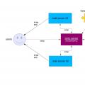 Email sending page Fill relay_recipients file with addresses from Active Directory
 Missing language bar in Windows - what to do?