Transmission function. Impulse response and transfer function Relationship of impulse response with transfer function
To determine the impulse response g(t, τ), where τ is the exposure time, t- the time of appearance and action of the response, it is necessary to use the differential equation of the circuit directly according to the given parameters of the circuit.
To analyze the method of finding g(t, τ), consider a simple chain described by a first-order equation:
where f(t) - impact, y(t) is the response.
A-priory, impulse response is the circuit response to a single delta pulse δ ( t-τ) supplied to the input at the moment t= τ. It follows from this definition that if on the right-hand side of the equation we put f(t)=δ( t-τ), then on the left you can accept y(t)=g(t,).
Thus, we arrive at the equation
 .
.
Because right part of this equation is equal to zero everywhere, except for the point t= τ, the function g(t) can be sought in the form of a solution to a homogeneous differential equation:

under the initial conditions following from the previous equation, as well as from the condition that by the moment of application of the impulse δ ( t-τ) there are no currents and voltages in the circuit.
The last equation separates the variables:


where  - the values of the impulse response at the time of exposure.
D  To determine the initial value
  back to the original equation. It follows from it that at the point
  function g(t) must jump by 1 / a 1 (τ), since only under this condition the first term in the original equation a 1 (t)[dg/dt] can form a delta function δ ( t-τ).
Since at 
 , then at the moment
 .
.
Replacing the indefinite integral with a definite one with a variable upper limit of integration, we obtain the relations for determining the impulse response:
Knowing the impulse response, it is easy to determine the transfer function of the linear parametric circuit, since both axes are connected by a pair of Fourier transforms:

where a=t-τ - signal delay. Function g 1 (t,a) is obtained from the function  by replacing τ = t-a.
Along with the last expression, another definition of the transfer function can be obtained, in which the impulse response g 1 (t,a) does not appear. To do this, we use the inverse Fourier transform for the response S OUT ( t):
 .
.
For the case where the input signal is harmonic, S(t) = cosω 0 t... Corresponding S(t) the analytical signal is  .
.
The spectral plane of this signal 
Substituting  instead of
  into the last formula, we get
From here we find:
Here Z OUT ( t) - analytical signal corresponding to the output signal S OUT ( t).
Thus, the output signal with harmonic action
is defined in the same way as for any other linear circuits.
If the transfer function K(jω 0 , t) changes in time according to a periodic law with the fundamental frequency Ω, then it can be represented as a Fourier series:
where  - time-independent coefficients, in the general case, complex, which can be interpreted as transfer functions of some two-port networks with constant parameters.
Work
can be considered as the transfer function of a cascade (series) connection of two four-port networks: one with a transfer function  , independent of time, and the second with the transfer function
  , which changes in time, but does not depend on the frequency ω 0 of the input signal.
 Based on the last expression, any parametric circuit with periodically changing parameters can be represented as the following equivalent circuit:
Where is the process of formation of new frequencies in the spectrum of the output signal clear?
The analytical signal at the output will be equal
where φ 0, φ 1, φ 2 ... are the phase characteristics of the two-port networks.
Passing to the real signal at the output, we get

This result indicates the following property of a circuit with variable parameters: when the transfer function changes according to any complex but periodic law with the fundamental frequency
Ω, a harmonic input signal with frequency ω 0 forms a spectrum at the output of the circuit containing frequencies ω 0, ω 0 ± Ω, ω 0 ± 2Ω, etc.
If a complex signal is applied to the input of the circuit, then everything said above applies to each of the frequencies ω and to the input spectrum. Of course, in a linear parametric circuit, there is no interaction between the individual components of the input spectrum (the principle of superposition) and frequencies of the form n ω 1 ± mω 2 where ω 1 and ω 2 are different frequencies of the input signal.
2.3 General properties of the transfer function.
The stability criterion for a discrete circuit coincides with the stability criterion for an analog circuit: the poles of the transfer function must be located in the left half-plane of the complex variable, which corresponds to the position of the poles within the unit circle of the plane
Chain transfer function general view is written, according to (2.3), as follows:
where the signs of the terms are taken into account in the coefficients a i, b j, while b 0 = 1.
It is convenient to formulate the properties of the transfer function of a chain of general form in the form of requirements for the physical realizability of a rational function of Z: any rational function of Z can be realized as a transfer function of a stable discrete chain up to a factor H 0 ЧH Q, if this function satisfies the requirements:
1.coefficients a i, b j are real numbers,
2.the roots of the equation V (Z) = 0, i.e. the poles of H (Z) are located within the unit circle of the Z plane.
The factor H 0 ЧZ Q takes into account the constant amplification of the signal H 0 and the constant shift of the signal along the time axis by the value of QT.
2.4 Frequency characteristics.
Discrete circuit transfer function complex
defines the frequency characteristics of the circuit
Frequency response, - phase frequency response.
Based on (2.6), the transfer function complex of general form can be written as
Hence the formulas for frequency response and phase frequency response
Frequency characteristics of a discrete circuit are periodic functions. The repetition period is equal to the sampling rate w d.
Frequency characteristics are usually normalized along the frequency axis to the sampling frequency
where W is the normalized frequency.
In calculations with the use of a computer, frequency normalization becomes a necessity.
Example. Determine the frequency characteristics of the circuit, the transfer function of which
H (Z) = a 0 + a 1 ЧZ -1.
Transfer function complex: H (jw) = a 0 + a 1 e -j w T.
taking into account the frequency normalization: wT = 2p H W.
H (jw) = a 0 + a 1 e -j2 p W = a 0 + a 1 cos 2pW - ja 1 sin 2pW.
Frequency response and phase response formulas
H (W) =, j (W) = - arctan ![]() .
.
frequency response and phase frequency response graphs for positive values a 0 and a 1 under the condition a 0> a 1 are shown in Fig. (2.5, a, b.)
Logarithmic scale of frequency response - attenuation A:
![]() ;
; ![]() . (2.10)
. (2.10)
The transfer function zeros can be located at any point of the Z plane. If the zeros are located within the unit circle, then the frequency response and phase response characteristics of such a circuit are related by the Hilbert transformation and can be uniquely determined one through the other. Such a circuit is called a minimum phase type circuit. If at least one zero appears outside the unit circle, then the chain belongs to a nonlinear-phase type chain for which the Hilbert transform is not applicable.
2.5 Impulse response. Convolution.
The transfer function characterizes the circuit in the frequency domain. In the time domain, the circuit is characterized by an impulse response h (nT). The impulse response of a discrete circuit is the circuit's response to a discrete d - function. Impulse response and transfer function are system characteristics and are linked by Z-conversion formulas. Therefore, the impulse response can be considered as a certain signal, and the transfer function H (Z) - Z is an image of this signal.
The transfer function is the main characteristic in the design, if the norms are set relative to the frequency characteristics of the system. Accordingly, the main characteristic is the impulse response if the norms are set in time.
The impulse response can be determined directly from the circuit as the circuit's response to the d - function, or by solving the difference equation of the circuit, assuming x (nT) = d (t).
Example. Determine the impulse response of the circuit, the diagram of which is shown in Figure 2.6, b.
The difference equation of the chain y (nT) = 0.4 x (nT-T) - 0.08 y (nT-T).
Solution of the difference equation in numerical form, provided that x (nT) = d (t)
n = 0; y (0T) = 0.4 x (-T) - 0.08 y (-T) = 0;
n = 1; y (1T) = 0.4 x (0T) - 0.08 y (0T) = 0.4;
n = 2; y (2T) = 0.4 x (1T) - 0.08 y (1T) = -0.032;
n = 3; y (3T) = 0.4 x (2T) - 0.08 y (2T) = 0.00256; etc. ...
Hence h (nT) = (0; 0.4; -0.032; 0.00256; ...)
For a stable circuit, the counts of the impulse response tend to zero over time.
The impulse response can be determined from a known transfer function by applying
a. inverse Z-transform,
b. decomposition theorem,
v. the lag theorem for the results of dividing the numerator polynomial by the denominator polynomial.
The last of the listed methods refers to the numerical methods for solving the problem.
Example. Determine the impulse response of the circuit in Fig. (2.6, b) by the transfer function.
Here H (Z) = ![]() .
.
Divide the numerator by the denominator

Applying the delay theorem to the result of division, we obtain
h (nT) = (0; 0.4; -0.032; 0.00256; ...)
Comparing the result with the calculations using the difference equation in the previous example, one can be convinced of the reliability of the calculation procedures.

It is proposed to determine independently the impulse response of the circuit in Fig. (2.6, a), applying successively both considered methods.
In accordance with the definition of the transfer function, Z - the image of the signal at the output of the circuit can be defined as the product of Z - the image of the signal at the input of the circuit and the transfer function of the circuit:
Y (Z) = X (Z) ЧH (Z). (2.11)
Hence, by the convolution theorem, the convolution of the input signal with an impulse response gives the signal at the output of the circuit
y (nT) = x (kT) Чh (nT - kT) = h (kT) Чx (nT - kT). (2.12)
Determination of the output signal by the convolution formula finds application not only in computational procedures, but also as an algorithm for the functioning of technical systems.
Determine the signal at the output of the circuit, the diagram of which is shown in Fig. (2.6, b), if x (nT) = (1.0; 0.5).
Here h (nT) = (0; 0.4; -0.032; 0.00256; ...)
Calculation according to (2.12)
n = 0: y (0T) = h (0T) x (0T) = 0;
n = 1: y (1T) = h (0T) x (1T) + h (1T) x (0T) = 0.4;
n = 2: y (2T) = h (0T) x (2T) + h (1T) x (1T) + h (2T) x (0T) = 0.168;
Thus, y (nT) = (0; 0.4; 0.168; ...).
In technical systems, instead of linear convolution (2.12), circular or cyclic convolution is more often used.


Student of group 220352 Chernyshev D. A. Reference - report on patent and scientific and technical research Topic of the final qualification work: television receiver with digital signal processing. Start of search 2. 02. 99. End of search 25.03.99 Search subject Country, Index (MKI, NKI) No ...


Carriers and single sideband amplitude phase modulation (AFM-SSB). 3. The choice of the duration and the number of elementary signals used to form the output signal In real communication channels for transmitting signals over frequency limited channel a signal of the form is used, but it is infinite in time, so it is smoothed according to the cosine law. , where - ...
This dynamic characteristic is used to describe single-channel systems.
with zero initial conditions
Transient response h (t) is the response of the system to the input single step action at zero initial conditions.

The moment of occurrence of the input action
Figure 2.4. System transient response
Example 2.4:
Transient characteristics for different values of active resistance in electrical circuit:
 | ||
To determine the transient response analytically, you must solve the differential equation with zero initial conditions and u (t) = 1 (t).
For a real system, the transient response can be obtained experimentally; in this case, a stepwise action should be applied to the input of the system and the response at the output should be recorded. If the step action is different from unity, then the output characteristic should be divided by the magnitude of the input action.
Knowing the transient response, it is possible to determine the response of the system to an arbitrary input action using the convolution integral
With the help of the delta function, the real input action of the impact type is simulated.

Figure 2.5. System impulse response
Example 2.5:
Impulse characteristics for different values of active resistance in the electrical circuit:
The transition function and impulse function are uniquely related to each other by the relations
Transition matrix is the solution to the matrix differential equation
Knowing the transition matrix, it is possible to determine the response of the system
![]()
on an arbitrary input action for any initial conditions x (0) by expression
If the system has zero initial conditions x (0) = 0, then
 , ,
| (2.17) |
For linear systems with constant parameters, the transition matrix Ф (t) is a matrix exponent
For small dimensions or simple matrix structure A expression (2.20) can be used to accurately represent the transition matrix using elementary functions. In the case of a large matrix A existing programs should be used to calculate the matrix exponential.
Transmission function
Along with ordinary differential equations in theory automatic control various transformations are used. For linear systems, it is more convenient to write these equations in symbolic form using the so-called differentiation operator
which allows transforming differential equations as algebraic and introducing a new dynamic characteristic - transfer function.
Consider this transition for multichannel systems of the form (2.6)


Let's write the equation of state in symbolic form:
px = Ax + Bu,
which allows us to determine the state vector
It is a matrix with the following components:
 | (2.27) |
where ![]() - scalar transfer functions
, which represent the ratio of the output to the input in symbolic form with zero initial conditions
- scalar transfer functions
, which represent the ratio of the output to the input in symbolic form with zero initial conditions
Own transfer functions i-th channel are the components of the transfer matrix ![]() that are on the main diagonal. The components located above or below the main diagonal are called cross-link transfer functions
between channels.
that are on the main diagonal. The components located above or below the main diagonal are called cross-link transfer functions
between channels.
The inverse matrix is found by the expression
Example 2.6.
Determine the transfer matrix for the object
Let us use the expression for the transfer matrix (2.27) and find a preliminary inverse matrix (2.29). Here
![]()
The transposed matrix has the form
![]() a det (pI-A) = p -2p + 1,.
a det (pI-A) = p -2p + 1,.
where is the transposed matrix. As a result, we get the following inverse matrix:

and the transfer matrix of the object

Transfer functions are most often used to describe single-channel systems of the form
where is the characteristic polynomial.
Transfer functions are usually written in a standard form:
 , ,
| (2.32) |
where is the transmission coefficient;
The transfer matrix (transfer function) can also be determined using Laplace or Carson-Heaviside images. If we subject both sides of the differential equation to one of these transformations and find the relationship between the input and output quantities at zero initial conditions, we get the same transfer matrix (2.26) or function (2.31).
In order to further distinguish transformations of differential equations, we will use the following notation:
Differentiation operator;
Laplace transform operator.
Having received one of the dynamic characteristics of the object, you can determine all the others. The transition from differential equations to transfer functions and vice versa is carried out using the differentiation operator p.
Consider the relationship between transient characteristics and transfer function. The output variable is found through the impulse function in accordance with expression (2.10),

Let's subject him Laplace transform,
 ,
,
and get y (s) = g (s) u (s). From here we define the impulse function:
 | (2.33) |
Thus, the transfer function is the Laplace transform of the impulse function.
Example 2.7.
Determine the transfer function of the object, the differential equation of which has the form
Using the differentiation operator d / dt = p, we write the equation of the object in symbolic form
on the basis of which we determine the desired transfer function of the object
![]()
Modal characteristics
Modal characteristics correspond to the free component of the motion of the system (2.6) or, in other words, reflect the properties of an autonomous system of the type (2.12)
The system of equations (2.36) will have a nonzero solution with respect to if
| | (2.37) |
Equation (2.37) is called characteristic and has n-roots, which are called eigenvalues matrices A... Substituting the eigenvalues in (2.37), we obtain
![]() .
.
where are eigenvectors,
The set of eigenvalues and eigenvectors is system modal characteristics .
For (2.34), only the following exponential solutions can exist
To obtain the characteristic equation of the system, it is sufficient to equate the common denominator of the transfer matrix (transfer function) to zero (2.29).
Frequency characteristics
If a periodic signal of a given amplitude and frequency is applied to the input of the object, then the output will also be a periodic signal of the same frequency, but in the general case of a different amplitude with a phase shift. The relationship between the parameters of periodic signals at the input and output of the object is determined frequency characteristics ... They are most often used to describe single-channel systems:
and is presented in the form
| | (2.42) |
The components of the generalized frequency response have an independent meaning and the following names:
The frequency response by expression (2.42) can be plotted on the complex plane. In this case, the end of the vector corresponding to the complex number, when changing from 0 to, draws a curve on the complex plane, which is called amplitude-phase characteristic (AFH).

Figure 2.6. An example of the amplitude-phase characteristic of the system
Phase-frequency response (PFC)- graphical display of the dependence of the phase shift between the input and output signals depending on the frequency,
![]()
To determine the numerator and denominator W (j) decompose into factors not higher than the second order
 ,
,
then ![]() where the "+" sign refers to i = 1,2, ..., l(the numerator of the transfer function), the sign "-" -к i = l + 1, ..., L(the denominator of the transfer function).
where the "+" sign refers to i = 1,2, ..., l(the numerator of the transfer function), the sign "-" -к i = l + 1, ..., L(the denominator of the transfer function).
Each of the terms is determined by the expression

Along with the AFC, all other frequency characteristics are plotted separately. So the frequency response shows how the link passes a signal of different frequencies; moreover, the estimate of the transmission is the ratio of the amplitudes of the output and input signals. The phase response shows the phase shifts introduced by the system at different frequencies.
In addition to the considered frequency characteristics, automatic control theory uses logarithmic frequency response ... The convenience of working with them is explained by the fact that the operations of multiplication and division are replaced by operations of addition and subtraction. The frequency response plotted on a logarithmic scale is called logarithmic frequency response (LACHH)
| , | (2.43) |
This value is expressed in decibels (db). When displaying the LFCH, it is more convenient to plot the frequency on the abscissa axis on a logarithmic scale, that is, expressed in decades (dec).

Figure 2.7. An example of a logarithmic amplitude frequency response
The phase-frequency characteristic can also be plotted on a logarithmic scale:

Figure 2.8. Example of a logarithmic phase frequency response
Example 2.8.
LFC, real and asymptotic LFC of the system, the transfer function of which has the form:
| | (2.44) |
 .
.
Rice. 2.9. Real and asymptotic LFC of the system
 .
.
Rice. 2.10. LFH systems
STRUCTURAL METHOD
3.1. Introduction
3.2. Proportional link (amplifying, inertialess)
3.3. Differentiating link
3.4. Integrating link
3.5. Aperiodic link
3.6. Forcing link (proportional - differentiating)
3.7. 2nd order link
3.8. Structural transformation
3.8.1. Serial connection of links
3.8.2. Parallel link connection
3.8.3. Feedback
3.8.4. Transfer rule
3.9. Transition from transfer functions to equations of state using structural diagrams
3.10. Scope of the structural method
Introduction
To calculate various automatic control systems, they are usually divided into separate elements, the dynamic characteristics of which are differential equations of no higher than second order. Moreover, elements that are different in their physical nature can be described by the same differential equations, therefore they are attributed to certain classes, called typical links .
An image of a system in the form of a set of typical links with an indication of the connections between them is called a structural diagram. It can be obtained both on the basis of differential equations (Section 2) and transfer functions. This method and constitutes the essence of the structural method.
Let us first consider in more detail the typical links that make up the automatic control systems.
Proportional link
(amplifying, inertialess)
Proportional is called the link, which is described by the equation
and the corresponding structural scheme is shown in Fig. 3.1.
The impulse function is:
g (t) = k .
There are no modal characteristics (eigenvalues and eigenvectors) for the proportional link.
Replacing in the transfer function p on j we get the following frequency characteristics:
Amplitude frequency response (AFC) is determined by the ratio:
This means that the amplitude of the periodic input signal is amplified by k- times, and there is no phase shift.
Differentiating link
Differentiating the link is called, which is described by the differential equation:
| y = k. | (3.6) |
Its transfer function is:
We now obtain the frequency characteristics of the link.
AFH : W (j) = j k, coincides with the positive imaginary semiaxis on the complex plane;
HFC: R () = 0,
MChH: I () = k,
Frequency response: ,
PFC:, that is, for all frequencies, the link introduces a constant phase shift;
Integrating link
This is a link, the equation of which is:
and then to its transfer function
Let us determine the frequency characteristics of the integrating link.
 | AFH:  ; HFC:; MFC: ; HFC:; MFC:  ; ;
it looks like a straight line on a plane (Figure 3.9). |
Characteristic equation
A (p) = p = 0
has a single root, which is the modal characteristic of the integrating link.
Aperiodic link
Aperiodic is called a link, the differential equation of which has the form
where, is the transmission coefficient of the link.
Replacing in (3.18) d / dt on p, we pass to the symbolic notation of the differential equation,
| (Tp + 1) y = ku, | (3.19) |
and define the transfer function of the aperiodic link:) = 20lg (k).
Impulse (weight) characteristic or impulse function
chains
- this is its generalized characteristic, which is a time function, numerically equal to the reaction of the circuit to a single impulse action at its input at zero initial conditions (Fig. 13.14); in other words, this is the response of the circuit, free from the initial supply of energy, to the Diran delta function  at its entrance.
|
|

Function  can be determined by calculating the transition
  or gear
  chain function.
Function calculation  using the transient function of the circuit. Let at the input action
  the reaction of a linear electric circuit is
  ... Then, due to the linearity of the circuit at the input action equal to the derivative
  , the chain reaction will be equal to the derivative
  .
.
As noted, at  , chain reaction
  , what if
  , then the chain reaction will be
  , i.e. impulse function
According to the sampling property  work
work  ... Thus, the impulse function of the circuit
 .
(13.8)
.
(13.8)
If  , then the impulse function has the form
 .
(13.9)
.
(13.9)
Consequently, the dimension of the impulse response is equal to the dimension of the transient response divided by time.
Function calculation  using the chain transfer function. According to expression (13.6), when acting on the input of the function
  , the response of the function will be the transient function
  kind:
kind:
 .
.
On the other hand, it is known that the image of the time derivative of a function  , at
, at  , is equal to the product
  .
.
Where  ,
,
or  ,
(13.10)
,
(13.10)
those. impulse response
 circuit is equal to the inverse Laplace transform of its transmission
 functions.
Example. Let us find the impulse function of the circuit, the equivalent circuits of which are shown in Fig. 13.12, a; 13.13.
Solution
The transition and transfer functions of this circuit were obtained earlier:

Then, according to expression (13.8)
where  .
.
|
|

Impulse response graph  circuit is shown in Fig. 13.15.
conclusions
Impulse response  introduced for the same two reasons as the transient response
  .
.
1. Single impulse action  - an abrupt and therefore quite heavy external influence for any system or circuit. Therefore, it is important to know the reaction of a system or a chain precisely under such an action, i.e. impulse response
  .
.
2. With the help of some modification of the Duhamel integral, one can, knowing  calculate the response of the system or circuit to any external disturbance (see further Sections 13.4, 13.5).
4. Integral overlay (Duhamel).
Let an arbitrary passive two-terminal network (Fig.13.16, a) connects to a source that is continuously changing from the moment  stresses
  (fig.13.16, b).
|
|

It is required to find the current  (or voltage) in any branch of the two-pole after the key is closed.
We will solve the problem in two stages. First, we find the desired value when the two-terminal network is turned on for a single voltage jump, which is set by a single step function  .
.
It is known that the reaction of a chain to a unit jump is transient response (function)
 .
.
For example, for  - circuit current transient function
  (see clause 2.1), for
  - circuit voltage transient function
  .
.
At the second stage, the continuously changing voltage  replace with a step function with elementary rectangular jumps
  (see fig.13.16 b). Then the process of voltage change can be represented as switching on at
  constant voltage
  , and then as the inclusion of elementary constant voltages
  offset relative to each other by time intervals
  and having a plus sign for the increasing and minus for the falling branch of the given voltage curve.
The component of the required current at the moment  from constant voltage
  is equal to:
 .
.
The component of the required current from an elementary voltage jump  included at the moment of time
  is equal to:
 .
.
Here, the argument of the transition function is time  , since the elementary voltage jump
  begins to act for a while
  later than the closure of the key, or, in other words, since the time interval between the moment
  the beginning of the action of this jump and the moment of time
  is equal to
  .
.
Elementary voltage surge
 ,
,
where  - scale factor.
Therefore, the sought-for component of the current
Elementary voltage surges are switched on in the time interval from  until the moment
  , for which the sought current is determined. Therefore, summing up the components of the current from all the jumps, passing to the limit at
  , and taking into account the current component from the initial voltage jump
  , we get:
The last formula for determining the current with a continuous change in the applied voltage
 (13.11)
called integral of superposition (superposition) or the Duhamel integral (the first form of writing this integral).
The problem is solved in a similar way when the circuit is connected to the current source. According to this integral, the reaction of the chain, in general form,  at some point
  after the start of exposure
  is determined by all that part of the impact that took place up to the point in time
  .
.
By substituting variables and integrating by parts, we can obtain other forms of writing the Duhamel integral, equivalent to expression (13.11):

The choice of the notation form for the Duhamel integral is determined by the convenience of the calculation. For example, if  is expressed by an exponential function, formula (13.13) or (13.14) turns out to be convenient, which is due to the simplicity of differentiating the exponential function.
At  or
or  it is convenient to use the notation in which the term before the integral vanishes.
Arbitrary impact  can also be represented as a sum of pulses connected in series, as shown in Fig. 13.17.
|
|

With an infinitely short pulse duration  we obtain the Duhamel integral formulas similar to (13.13) and (13.14).

The same formulas can be obtained from relations (13.13) and (13.14), replacing the derivative of the function  impulse function
  .
.
Output.
Thus, based on the Duhamel integral formulas (13.11) - (13.16) and the time characteristics of the chain  and
and  the timing functions of the circuit responses can be defined
  on arbitrary influences
  .
.
Let an arbitrary impulse system be given by a structural diagram, which is a set of standard connections from the simplest impulse systems (connections of the feedback type, serial and parallel). Then, in order to obtain the transfer function of this system, it is enough to be able to find the transfer function of standard connections from the transfer functions of the connected impulse systems, since the latter are known (either exactly or approximately) (see § 3.1).
Connections of purely impulse systems.
The formulas for calculating the -transfer functions of standard connections of purely impulsive systems in terms of the z-transfer functions of the connected purely impulsive elements coincide with similar formulas from the theory of continuous systems. This coincidence occurs because the structure of formula (3.9) coincides with the structure of a similar formula from the theory of continuous systems, formula (3.9) describes the operation of a purely impulsive system exactly.
An example. Find the z-transfer function of a purely impulse system given by the structural diagram (Fig. 3.2).
Taking into account (3.9) from the block diagram shown in Fig. 3.2, we get:

Substitute the last expression into the first:
![]()
(compare with the well-known formula from the theory of continuous systems).
Impulse system connections.
Example 3.2. Let the impulse system be represented by a structural diagram (see Fig. 3.3, excluding the dotted line and dash-dotted line). Then

If you need to determine the discrete values of the output (see the fictitious synchronous key at the output - the dotted line in Fig. 3.3), then in a manner similar to that used to derive (3.7), we get the connection:


Consider another system (Fig. 3.4, excluding the dotted line), which differs from the previous one only in the location of the key. For her

With a fictitious key (see the dotted line in Fig. 3.4)
From the relationships obtained in this example, conclusions can be drawn.
Conclusion 1. The type of analytical connection of the input as with continuous [see. (3.10), (3.12)] and with discrete [cf. (3.11), (3.13)] by the values of the output of an arbitrary impulsive system essentially depends on the location of the key.
Conclusion 2. For an arbitrary impulse system, as well as for the simplest one, which is described in 3.1, it is not possible to obtain a characteristic similar to the transfer function that connects the input and output at all times. It is not possible to obtain a similar characteristic that connects the input and output and at discrete times, multiples, which was done for the simplest impulse system (see § 3.1). This can be seen from the relations (3.10), (3.12) and (3.11), (3.13), respectively.
Conclusion 3. For some special cases of connections of impulse systems, for example, for a impulse system, the structural diagram of which is shown in Fig. 3.5 (no dotted line), it is possible to find a transfer function connecting the input and output at discrete times, multiples. Indeed, from (3.10) at follows But then [see derivation of formula (3.7)]
Communication structure z-transfer function open and closed systems in this case is the same as in the theory of continuous systems.
It should be noted that although this is a special case, it is of very great practical importance, since many systems from the class of pulse tracking systems are reduced to it.
Conclusion 4. To obtain a convenient expression similar to the z-transfer function in the case of an arbitrary impulse system (see, for example, Fig. 3.3), it is required to introduce synchronous dummy keys not only at the output of the system (see the dotted line in Fig. 3.3), but and at its other points (see, for example, the dash-dotted section instead of the solid one in Fig. 3.3). Then
and formulas (3.10), (3.11) take the following form, respectively:
and therefore
![]()
The consequences of introducing the keys shown in Fig. 3.3 with a dash-dot line and a dotted line are significantly different, since the latter does not change the nature of the operation of the entire system, it simply gives information about it at discrete times.

The first, converting into a pulse that continuous signal that goes to the link feedback, turns the original system into a completely different one. This new system will be able to represent the operation of the original system well enough if it is accepted (see § 5.4) and if
1) the conditions of the Kotelnikov theorem (2.20) are satisfied;
2) the bandwidth of the feedback link is less:
![]()
where is the cutoff frequency of the feedback link;
3) the amplitude frequency response (AFC) of the link in the region of the cutoff frequency decreases quite steeply (see Fig. 3.6).

Then only that part of the pulse signal spectrum that corresponds to the continuous signal passes through the feedback link.
Thus, formula (3.16) in the general case only approximately represents the work of the original system even at discrete times. Moreover, it does this the more accurately, the more reliably conditions (2.20), (3.17) and the conditions of a steep fall of the amplitude-frequency characteristic for a link, the normal operation of which is violated by a fictitious key, are satisfied.
So, using the z-transform, you can accurately investigate the operation of a purely impulsive system; using the Laplace transform - to accurately investigate the operation of a continuous system.
An impulse system with the help of one (any) of these transformations can be investigated only approximately, and even then under certain conditions. The reason for this is the presence in a pulse system of both continuous and pulse signals (therefore, such pulse systems are continuous pulse and are sometimes called continuous-discrete). In this regard, the Laplace transform, which is convenient when operating with continuous signals, becomes inconvenient when it comes to discrete signals... Convenient for discrete signals, z-transformation is inconvenient for continuous ones.


So in this case, the noted in the aporias is manifested)
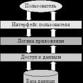 Architecture of a distributed control system based on a reconfigurable multi-pipeline computing environment L-Net "transparent" distributed file systems
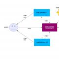 Email sending page Fill relay_recipients file with addresses from Active Directory
 Missing language bar in Windows - what to do?